DuckDB Internals: Why is DuckDB Fast? (Part 1)DuckDB 内部原理：DuckDB 为什么快？（第一部分）

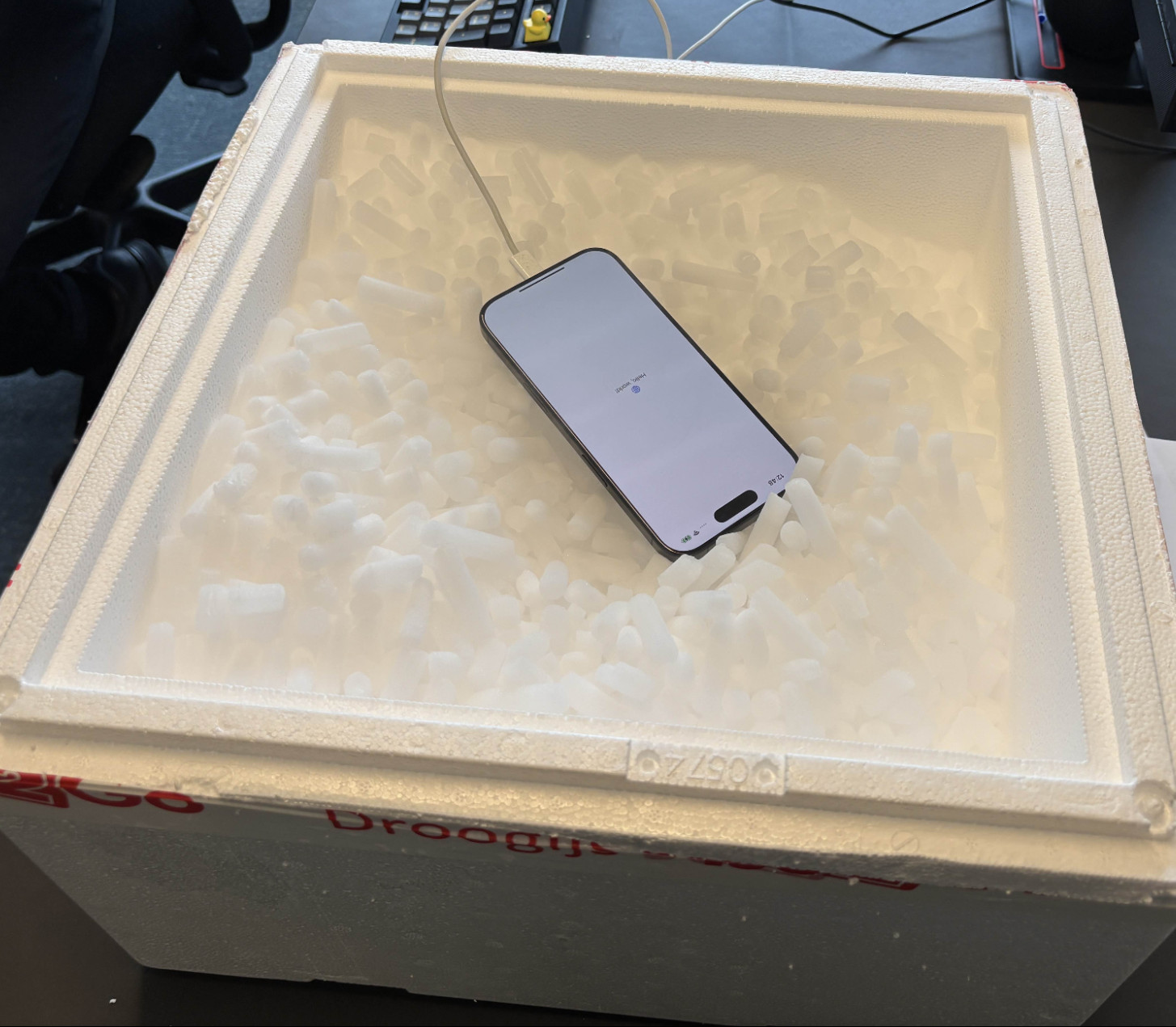
DuckDB has gone from a research project at CWI Amsterdam in 2019 to one of the most widely adopted databases of the past decade. The list of places it shows up is long: notebooks, ETL pipelines, dashboards, CI test runners, embedded analytics inside SaaS products, even an iPhone running TPC-H at scale factor 100.DuckDB 从 2019 年在阿姆斯特丹 CWI 的研究项目，发展为过去十年中最广泛采用的数据库之一。它出现的场景非常多：笔记本、ETL 流程、仪表盘、CI 测试运行器、SaaS 产品中的嵌入式分析，甚至还有在 iPhone 上运行规模因子 100 的 TPC‑H。

Companies have started building real products around it. MotherDuck is wrapping DuckDB into a cloud data warehouse. BI and data app platforms like Hex, Omni, and Evidence use it as an in-app execution engine and cache. Fivetran's Managed Data Lake Service uses DuckDB inside its data-lake writer for merging and compaction. Rill builds an open-source BI tool on top of it. We use it at Greybeam too, powering millions of queries for BI and analytics workloads.公司已经开始围绕它构建真实产品。MotherDuck 将 DuckDB 包装成云数据仓库。Hex、Omni、Evidence 等 BI 与数据应用平台将其作为应用内执行引擎和缓存。Fivetran 的托管数据湖服务在其数据湖写入器中使用 DuckDB 进行合并和压缩。Rill 在其之上构建开源 BI 工具。我们在 Greybeam 也使用它，为 BI 与分析工作负载提供数百万查询的动力。

What is DuckDB?#什么是 DuckDB？#

DuckDB is an in-process analytical SQL database. Analytical means it's optimized for the kind of queries that scan millions of rows to filter, aggregate, and join — not the kind that look up a single record by primary key. In-process means there's no server. You don't connect to DuckDB; you load it as a library inside your program, the same way you'd load NumPy or Polars.DuckDB 是一种进程内分析型 SQL 数据库。分析型意味着它针对需要扫描数百万行进行过滤、聚合和连接的查询进行优化——而不是通过主键查找单条记录的查询。进程内意味着没有服务器。你不需要连接到 DuckDB；只需像加载 NumPy 或 Polars 那样，将其作为库加载到你的程序中。

DuckDB has received widespread adoption because it's just so damn easy to use. It ships as a single binary under 20 MB with no external dependencies. You install it with pip install duckdb, brew install duckdb, or by linking libduckdb into a C++ project. It opens any directory of Parquet, CSV, or JSON files like they were already a SQL database.DuckDB 之所以被广泛采用，正是因为它极其易用。它以单个不到 20 MB 的二进制文件发布，无需外部依赖。你可以通过 `pip install duckdb`、`brew install duckdb`，或在 C++ 项目中链接 `libduckdb` 来安装。它可以像已经是 SQL 数据库一样打开任意目录下的 Parquet、CSV 或 JSON 文件。

DuckDB also happens to be one of the fastest single-node analytical engines available, regularly holding its own against entire clusters that cost millions of dollars per year.DuckDB 还是目前最快的单节点分析引擎之一，常常能够与每年花费数百万美元的整套集群相媲美。

This is the first post in a three-part deep dive into DuckDB internals. We'll follow a query from the moment it enters the engine to the moment the result is returned, and at each stage we'll look at the design choice that makes it fast. 这是关于 DuckDB 内部原理的三部分深度解析的第一篇。我们将从查询进入引擎的那一刻跟踪到结果返回的那一刻，并在每个阶段查看让它快速的设计选择。

DuckDB's speed comes from a handful design choices:DuckDB 的速度来源于以下几个设计选择：

1. In-process execution进程内执行
2. Columnar, compressed storage with zonemaps列式、压缩存储并带有分区映射（zonemaps）
3. Vectorized execution向量化执行
4. Morsel-driven parallelism基于 morsel 的并行化
5. Snapshot isolation with optimistic MVCC乐观 MVCC 的快照隔离
6. And much more!以及更多！

This post covers the path from your SQL to the moment the engine is ready to run the query, plus the storage layer the query will read from. By the end you'll have a clear mental model of DuckDB's setup work and storage layout. Query execution is covered in Part 2 so make sure to subscribe!本文覆盖了从你的 SQL 到引擎准备运行查询的路径，以及查询将读取的存储层。阅读完后，你将对 DuckDB 的准备工作和存储布局有清晰的心智模型。查询执行将在第 2 部分介绍，请务必订阅！

Queries Run In-Process#查询在进程内运行#

You point DuckDB at a 6 GB Parquet file on your laptop. The results come back in under a second. No cluster, no setup, no migration, no CREATE TABLE. How does that work?你在笔记本上指向一个 6 GB 的 Parquet 文件。结果在不到一秒的时间返回。没有集群、没有设置、没有迁移、没有 CREATE TABLE。它是怎么做到的？

SELECT
  *
FROM 'orders.parquet';

Most analytical databases are servers. Snowflake, Postgres, BigQuery, Redshift. You open a connection, send SQL over TCP (a protocol to send data over a network), and wait for results to come back. Along the way, every record in the result is serialized into a wire protocol, transmitted across the network, and deserialized on the other end.大多数分析数据库都是服务器模式。Snowflake、Postgres、BigQuery、Redshift。你打开一个连接，通过 TCP（网络传输协议）发送 SQL，然后等待结果返回。期间，结果中的每条记录都会被序列化为网络协议格式，跨网络传输，再在另一端反序列化。

Serializing and Deserializing#序列化与反序列化#

Inside a database, a query result lives as typed values at specific memory addresses. A 64-bit integer here, a pointer to a string there. Those addresses only exist in that process. To send the result to a client on another machine, the database has to rewrite every value into an agreed byte format (Postgres has its own, MySQL has another, with ODBC and JDBC as client-side APIs that drivers expose on top) so it can be pushed through a TCP socket. The client then parses those bytes back into its own native types. Every value may be touched multiple times, once to encode and once to decode, and on a large result set, that work often takes longer than the query itself.在数据库内部，查询结果以特定内存地址上的类型化值存在。这里是 64 位整数，那里是指向字符串的指针。这些地址只在该进程内有效。要把结果发送到另一台机器的客户端，数据库必须把每个值重新写成约定的字节格式（Postgres 有自己的格式，MySQL 有另一种，ODBC 与 JDBC 作为客户端 API 在驱动上实现），然后通过 TCP 套接字发送。客户端再把这些字节解析回自己的本地类型。每个值会被触碰两次：一次编码，一次解码，在大结果集上，这些工作往往比实际查询本身更耗时。

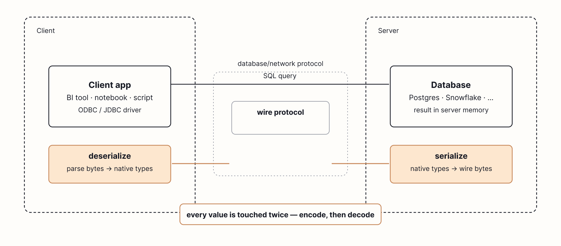
DuckDB is not a server. It's a library. There is no DuckDB daemon, no port, no cluster. You load libduckdb into your program and call functions directly against it.DuckDB 不是服务器，它是一个库。没有 DuckDB 守护进程、没有端口、没有集群。你把 libduckdb 加载到程序中，直接调用函数。

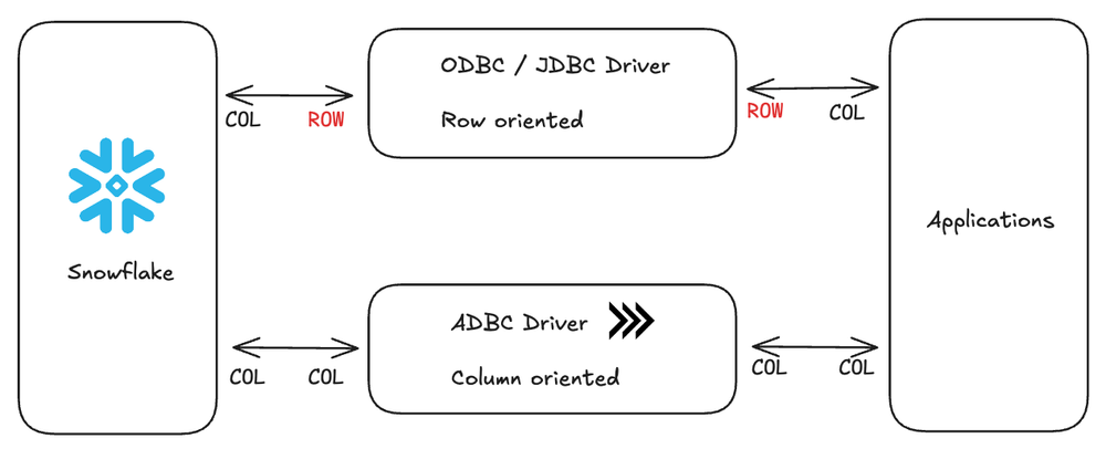
In 2017, Mark Raasveldt and Hannes Mühleisen published Don't Hold My Data Hostage, a paper measuring what actually happens when you pull a result set out of a warehouse. They found that the client protocol itself — ODBC, JDBC, and similar row-by-row value APIs — was often the slowest single step in the entire query, sometimes dwarfing the time the database spent computing the answer.2017 年，Mark Raasveldt 与 Hannes Mühleisen 发表了《Don't Hold My Data Hostage》论文，测量了从仓库中提取结果集时实际发生的情况。他们发现客户端协议本身——ODBC、JDBC 以及类似的逐行值 API——往往是整个查询中最慢的单一步骤，有时甚至超过数据库计算答案的时间。

Two costs drive this. The first is raw bandwidth: a typical gigabit Ethernet link caps you at around 125 MB/s, and a large result set can take longer to transmit than it took to compute. The second is per-value overhead. ODBC and JDBC hand back results one row and one value at a time, which means the client makes a separate function call for every field in every row. On a 100-million-row result, that's hundreds of millions of function calls, each one doing its own little memory copy, type check, and string allocation.这背后有两类成本。第一是原始带宽：典型的千兆以太网链路上限约为 125 MB/s，大结果集的传输时间可能比计算时间更长。第二是每个值的开销。ODBC 与 JDBC 逐行返回结果，这意味着客户端为每行的每个字段都要进行一次函数调用。对 1 亿行的结果来说，这意味着数亿次函数调用，每次都要进行内存拷贝、类型检查和字符串分配。

ADBC transfers data between systems in columnar Arrow format, which avoids the row-by-row serialization/deserialization that ODBC and JDBC require. Our friends at Columnar are making this commonplace.ADBC 以列式 Arrow 格式在系统之间传输数据，避免了 ODBC 与 JDBC 所需的逐行序列化/反序列化。我们的朋友们在 Columnar 正在让这成为常态。

DuckDB sidesteps both bottlenecks by living in the same process as the client.DuckDB 通过与客户端处于同一进程中，规避了这两个瓶颈。

When a Python script runs con.sql("SELECT ... FROM my_df") against a pandas dataframe, DuckDB can use a feature called a replacement scan. Instead of copying the dataframe into an internal table first, DuckDB replaces the table reference with a function that reads from the dataframe when the query runs.当 Python 脚本对 pandas DataFrame 执行 `con.sql("SELECT ... FROM my_df")` 时，DuckDB 可以使用一种称为 replacement scan 的特性。它不是先把 DataFrame 复制到内部表，而是把表引用替换为在查询运行时读取 DataFrame 的函数。

In the best case, DuckDB can read the same underlying buffers the Python process already owns, so it avoids materializing a second full copy of the data. This is zero-copy! If NumPy says "here's a buffer (contiguous chunk of memory) of 1 million int64 values," DuckDB can often read that same buffer directly because it understands the same physical layout. 在最佳情况下，DuckDB 可以直接读取 Python 进程已经拥有的底层缓冲区，从而避免对数据进行第二次完整拷贝。这就是零拷贝！如果 NumPy 说“这里有一个包含 100 万个 int64 值的缓冲区（连续内存块）”，DuckDB 往往可以直接读取该缓冲区，因为它理解相同的物理布局。

In practice, whether the path is truly zero-copy depends on the dataframe’s physical layout, column types, null representation, and string storage. If the types or layouts do not line up, DuckDB may allocate converted buffers for some columns.实际上，是否真的零拷贝取决于 DataFrame 的物理布局、列类型、空值表示以及字符串存储方式。如果类型或布局不匹配，DuckDB 可能会为某些列分配转换后的缓冲区。

Arrow is the cleanest version of this story because Arrow is already a columnar, typed memory format designed for sharing data between systems. That is why returning DuckDB results as Arrow, or querying Arrow-backed data, can avoid much of the row-by-row conversion overhead that traditional APIs impose.Arrow 是这个故事最干净的版本，因为 Arrow 本身就是一种列式、类型化的内存格式，专为系统间共享数据而设计。这也是为什么把 DuckDB 结果返回为 Arrow，或查询基于 Arrow 的数据，可以避免传统 API 带来的大量逐行转换开销。

From SQL to Logical Plan#从 SQL 到逻辑计划#

Once your SQL reaches DuckDB, it goes through the usual stages: parse, bind, plan, optimize.一旦你的 SQL 到达 DuckDB，它会经历常规的阶段：解析、绑定、计划、优化。

Parsing#解析#

The first step is to parse SQL into an abstract syntax tree (AST). DuckDB uses a fork of the Postgres parser, which is part of why DuckDB's dialect feels so familiar. 第一步是把 SQL 解析成抽象语法树（AST）。DuckDB 使用的是 Postgres 解析器的分支，这也是 DuckDB 方言如此熟悉的原因之一。

An AST is a tree representation of your query where each node is a syntactic construct: a SELECT statement, a column reference, a function call, a join, a literal. Parsing turns the flat string SELECT sum(l_quantity) FROM lineitem WHERE l_shipdate > '2024-01-01' into a structured object the engine can actually reason about.AST 是查询的树形表示，每个节点都是一种语法构造：SELECT 语句、列引用、函数调用、连接、字面量。解析把平铺的字符串 `SELECT sum(l_quantity) FROM lineitem WHERE l_shipdate > '2024-01-01'` 转换为引擎能够真正推理的结构化对象。

Select(
    expressions=[
        Sum(
            this=Column(
                this=Identifier(this=l_quantity, quoted=False)))],
    from_=From(
        this=Table(
            this=Identifier(this=lineitem, quoted=False))),
    where=Where(
        this=GT(
            this=Column(
                this=Identifier(this=l_shipdate, quoted=False)),
        expression=Literal(this='2024-01-01', is_string=True))))

A tree structure is what lets the rest of the engine do its job. The binder walks the nodes to resolve l_quantity to a specific column in a specific table. The optimizer pattern-matches subtrees to recognize that the WHERE predicate can be pushed down into the scan. The physical planner maps function call nodes to executable operators. None of these passes can operate on raw SQL. They need to traverse, pattern-match, and rewrite a typed structure. 树结构让引擎的其余部分得以工作。绑定器遍历节点，将 `l_quantity` 解析为特定表中的具体列。优化器对子树进行模式匹配，识别出 WHERE 谓词可以下推到扫描阶段。物理计划器把函数调用节点映射到可执行的算子。所有这些阶段都不能直接在原始 SQL 上操作，它们需要遍历、模式匹配并重写类型化结构。

Binding#绑定#

The next step is binding, which resolves every name in the AST against the catalog. lineitem becomes a specific table with a known schema. l_quantity becomes a specific column with a known type. sum becomes a specific aggregate function whose input type matches that column. Type checking happens here too: comparing l_shipdate to the string '2024-01-01' works because the binder coerces the literal to a date.下一步是绑定，它将 AST 中的每个名称解析到目录中。`lineitem` 成为具有已知模式的具体表，`l_quantity` 成为具有已知类型的具体列，`sum` 成为输入类型匹配该列的具体聚合函数。类型检查也在此进行：将 `l_shipdate` 与字符串 `'2024-01-01'` 比较能够成功，因为绑定器会把字面量强制转换为日期。

The output is a bound tree where every node knows what it refers to and what type it produces. Errors like unresolved columns, ambiguous references, and type mismatches surface at this stage.输出是一个已绑定的树，树中的每个节点都知道它引用的对象以及产生的类型。未解析的列、歧义引用和类型不匹配等错误会在此阶段显现。

At this point, DuckDB has turned raw SQL text into a typed tree. The engine no longer sees l_quantity as just a string in a query; it sees a specific column with a specific type from a specific table.此时，DuckDB 已经把原始 SQL 文本转化为类型化的树。引擎不再把 `l_quantity` 视为查询中的字符串，而是把它视为来自特定表的特定列及其类型。

The Optimizer#优化器#

In DuckDB, the optimizer consists of a sequence of small, focused transformations that you can, in fact, inspect and disable individually.在 DuckDB 中，优化器由一系列小而专注的转换组成，你实际上可以检查并单独禁用它们。

D SELECT * FROM duckdb_optimizers();
┌────────────────────────────┐
│            name            │
│          varchar           │
├────────────────────────────┤
│ expression_rewriter        │
│ filter_pullup              │
│ filter_pushdown            │
│ empty_result_pullup        │
│ cte_filter_pusher          │
│ regex_range                │
│ in_clause                  │
│ join_order                 │
│ deliminator                │
│ unnest_rewriter            │
│ unused_columns             │
│ statistics_propagation     │
│ common_subexpressions      │
│ common_aggregate           │
│ column_lifetime            │
│ limit_pushdown             │
│ row_group_pruner           │
│ top_n                      │
│ top_n_window_elimination   │
│ build_side_probe_side      │
│ compressed_materialization │
│ duplicate_groups           │
│ reorder_filter             │
│ sampling_pushdown          │
│ join_filter_pushdown       │
│ extension                  │
│ materialized_cte           │
│ sum_rewriter               │
│ late_materialization       │
│ cte_inlining               │
│ common_subplan             │
│ join_elimination           │
│ window_self_join           │
└────────────────────────────┘
           33 rows          

Running SET disabled_optimizers = 'filter_pullup, join_order' turns specific passes off so you can see what they were doing. 执行 `SET disabled_optimizers = 'filter_pullup, join_order'` 可以关闭特定的优化阶段，以观察它们的作用。

Here are a few interesting optimizers:以下是一些有趣的优化器：

Filter pushdown#过滤下推#

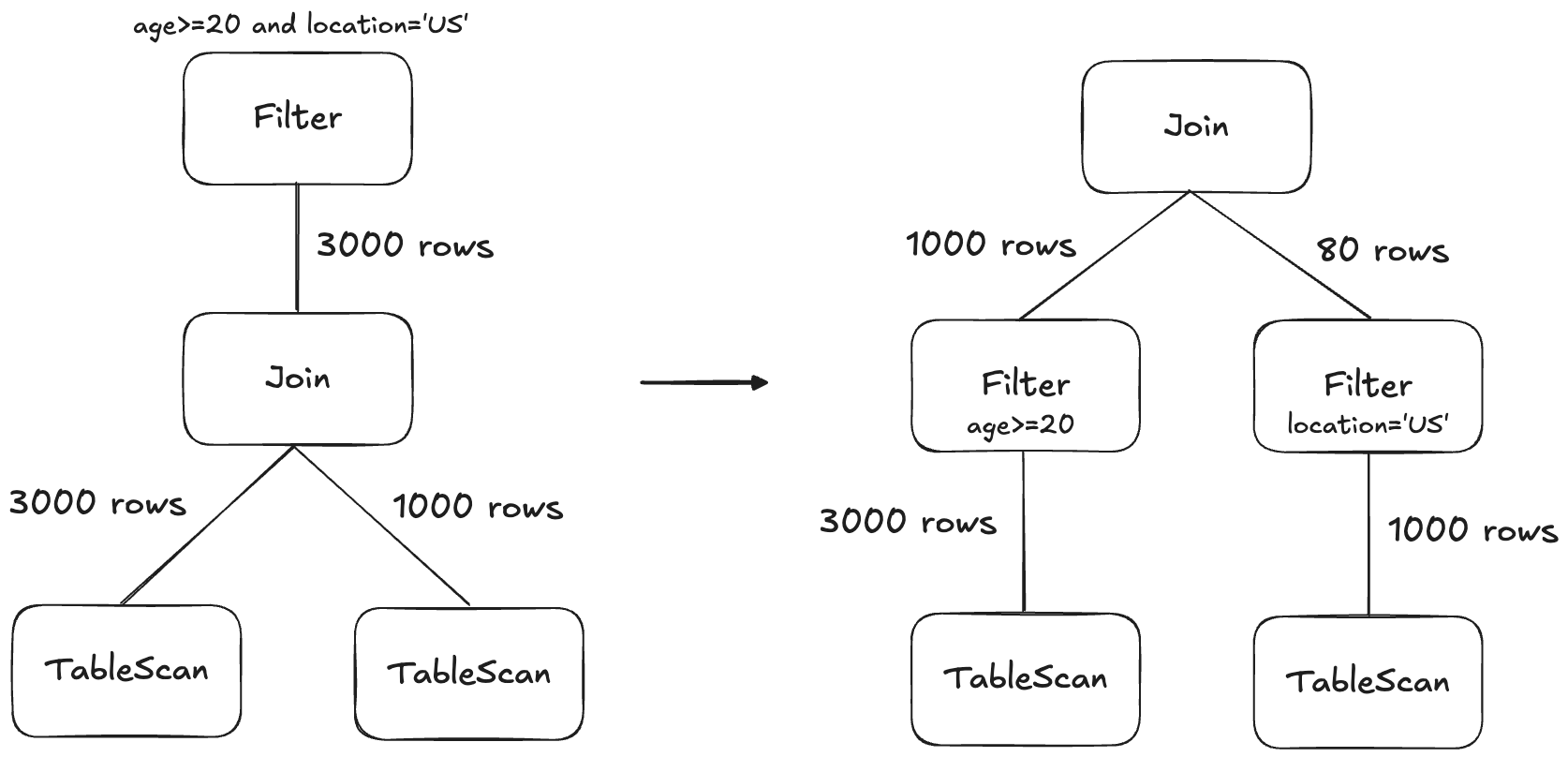
This is a classic database optimization: move WHERE predicates as close to the scan as possible so you prune data as early as possible. DuckDB first pulls filters up to the top of the plan so they can be combined and reorganized, then pushes them back down as far as possible.这是经典的数据库优化：尽可能把 WHERE 谓词移动到扫描阶段，以便尽早裁剪数据。DuckDB 先把过滤器提升到计划顶部，以便合并和重组，然后尽可能向下推。

Subquery unnesting#子查询去嵌套#

Correlated subqueries traditionally force a database to run the inner query once per outer row, which is slow. DuckDB implements techniques from the Unnesting Arbitrary Queries paper to rewrite these as joins, which are dramatically faster.相关子查询传统上会导致数据库对外层每行都执行一次内层查询，速度很慢。DuckDB 实现了《Unnesting Arbitrary Queries》论文中的技术，将其改写为连接，速度显著提升。

Dynamic join-filter pushdown#动态连接过滤下推#

During a hash join (more on hash joins here), the build side has to be fully read before the probe side starts. DuckDB takes advantage of that ordering: once the build side is in memory, it computes the min and max of the join key values it actually contains, then pushes those bounds back into the probe-side scan as a runtime filter. If the build side turned out to contain values only between 100 and 200, the probe scan can use the table's zonemaps to skip any row groups outside that range before reading them.在哈希连接期间（后文会详细介绍），构建端必须全部读取完毕后探测端才能开始。DuckDB 利用这一顺序：一旦构建端在内存中，就计算实际包含的连接键的最小值和最大值，然后把这些边界作为运行时过滤器推回探测端的扫描。如果构建端的键值仅在 100 到 200 之间，探测扫描可以利用表的分区映射（zonemap）跳过超出该范围的行组。

When the build side has fewer than 50 distinct join key values, the filter becomes an IN list instead of a min-max range, which is more precise and skips even more rows.当构建端的不同连接键值少于 50 个时，过滤器会变成 IN 列表而不是 min‑max 范围，精度更高，跳过的行更多。

Join order optimization#连接顺序优化#

Join order is the most consequential decision the optimizer makes. The order in which joins run determines how big each intermediate result is. A query joining six tables has 30,240 possible tree shapes, and the difference between best and worst can be orders of magnitude in runtime. Picking well requires estimating how many rows each candidate join will produce, which depends on table sizes, predicate selectivity, and the order of joins that came before.连接顺序是优化器最关键的决策。连接的执行顺序决定了每个中间结果的大小。一个涉及六个表的查询有 30,240 种可能的树形结构，最佳与最差之间的运行时间差距可能是数量级的。要做出良好选择，需要估算每个候选连接会产生多少行，这取决于表大小、谓词选择性以及之前的连接顺序。

DuckDB models the query as a graph. Each table is a node, and each join predicate is an edge connecting the tables it references. The optimizer's job is to pick an order to combine the nodes into a single tree, where each combination is a join. For example, if we have a query joining a to b , b to c, and c to d, the graph might look like this:DuckDB 将查询建模为图。每个表是一个节点，每个连接谓词是连接这些表的边。优化器的任务是挑选一种顺序，将节点组合成一棵树，每次组合对应一次连接。例如，如果我们有 a 与 b、b 与 c、c 与 d 的连接，图可能如下所示：

a ── b ── c ── d

To find the best tree, DuckDB uses dynamic programming, such as DPhyp or DPccp. Dynamic programming is a fancy name for a simple idea: if you've already figured out the best way to join {a, b, c}, you can reuse that answer when figuring out the best way to join {a, b, c, d}. You don't need to re-explore all the orderings inside {a, b, c} . It does this for every connected pair, then triplet, then quadruplet, etc. 为了找到最佳树，DuckDB 使用动态规划，例如 DPhyp 或 DPccp。动态规划本质上是一个简单的想法：如果你已经找到了连接 `{a, b, c}` 的最佳方式，那么在求 `{a, b, c, d}` 的最佳方式时可以复用这个答案。你不需要重新探索 `{a, b, c}` 内部的所有排列。它对每个已连接的对、三元组、四元组等都这样做。

There are dozens more optimizations to explore and the entire optimization phase usually finishes in about a millisecond. After optimization, DuckDB has a logical plan. The next step is to translate that plan into something the engine can actually execute.还有数十种其他优化，整个优化阶段通常在约一毫秒内完成。优化结束后，DuckDB 拥有逻辑计划。下一步是把该计划翻译成引擎实际可以执行的形式。

If you've enjoyed reading this so far, consider subscribing. We'll continue sharing more about the intricacies of DuckDB and many other query engines.如果你已经读到这里并觉得有收获，请考虑订阅。我们将继续分享 DuckDB 以及其他查询引擎的细节。

The Physical Plan#物理计划#

Imagine the optimizer hands the engine this plan, written in plain English:想象优化器把下面这段用普通英语写的计划交给引擎：

Read events from disk. Drop the rows where event_date is on or before 2026-01-01. Group what's left by customer_id and add up amount. Sort the result by total descending. Return the top 10.从磁盘读取事件。删除 event_date 在 2026‑01‑01 及之前的行。对剩余数据按 customer_id 分组并求和 amount。按 total 降序排序结果。返回前 10 条。

The engine now has to decide how to actually run those steps in a way that uses the CPU well and parallelizes across cores.引擎现在必须决定如何实际执行这些步骤，以充分利用 CPU 并在核心之间并行化。

Mapping Logical Steps to Physical Operators#将逻辑步骤映射到物理算子#

The optimizer's output is still a logical plan. It says what each step needs to compute but not which algorithm should do the computing. Most logical steps have several physical implementations.优化器的输出仍然是逻辑计划。它说明每一步需要计算什么，但没有指定使用哪种算法来完成计算。大多数逻辑步骤都有多种物理实现。

Take a join. The same logical join can be turned into any of: hash join, index join, piecewise merge join, cartesian join.以连接为例。相同的逻辑连接可以实现为：哈希连接、索引连接、分段合并连接、笛卡尔连接等。

DuckDB walks the logical plan and picks a physical operator for each node based on the shape of its inputs and predicates. The output is a physical plan — a tree of physical operators the executor knows how to run.DuckDB 遍历逻辑计划，根据输入的形状和谓词为每个节点挑选物理算子。输出是物理计划——执行器能够运行的物理算子树。

We will save the details of vectorized execution for Part 2, but one execution concept is useful now: the physical plan is not run as one giant tree walk. DuckDB breaks it into pipelines.我们将在第 2 部分保存向量化执行的细节，但现在有一个执行概念很有用：物理计划不会一次性作为完整的树遍历运行。DuckDB 会把它拆分为多个管道（pipeline）。

Pipelines#管道#

Think of a pipeline as an assembly line. Data enters at one end and passes through a chain of stations. Each station does one thing (drop a row, transform a column, look up a value in a hash table) and hands the result to the next station. As long as each station can decide what to do with a row using only that row, the line keeps moving. Examples of pipelines:把管道想象成装配线。数据从一端进入，经过一系列站点。每个站点只做一件事（丢弃一行、转换一列、在哈希表中查找一个值），然后把结果交给下一个站点。只要每个站点能够仅凭当前行决定如何处理，装配线就能持续前进。管道示例：

• WHERE: it either passes the row through or drops it. No state needed.WHERE：要么通过该行，要么丢弃。无需状态。
• A Projection: it computes new column values and emits them.投影：计算新列的值并输出。
• Probe side of hash join: once the hash table has been built, it looks up the row's key in the hash table and emits the joined row or nothing if no match.哈希连接的探测端：哈希表构建完成后，查找行的键并输出连接后的行，若无匹配则不输出。

In DuckDB, a connected chain of streaming stations like this is called a pipeline. Pipelines parallelize cleanly since every CPU core can run its own copy of the assembly line on its own slice of the input.在 DuckDB 中，这类相连的流式站点链称为管道。管道易于并行化，因为每个 CPU 核心可以在自己的输入切片上运行一条装配线的副本。

Pipeline breakers#管道阻断点#

Some operators can't work this way. They need to see the entire input before they can produce an output.有些算子无法这样工作。它们需要看到全部输入才能产生输出。

• ORDER BY can't emit a single sorted row until its seen every row because it doesn't know which row belongs first.ORDER BY 必须在看到所有行后才能输出已排序的行，因为它不知道哪一行应当排在最前。
• GROUP BY can't emit the final sum until it has accounted for every row in a grouping.GROUP BY 必须在处理完所有行后才能输出最终的求和结果。
• Build side of a hash join has to build the hash table before it can start looking anything up.哈希连接的构建端必须在开始查找之前先构建哈希表。

These operators are called pipeline breakers or sinks. They mark the end of one pipeline and the beginning of the next. The physical plan is effectively a sequence of pipelines stitched together by sinks.这些算子被称为管道阻断点或 sink。它们标记了一个管道的结束和下一个管道的开始。物理计划实际上是一系列由 sink 串联的管道。

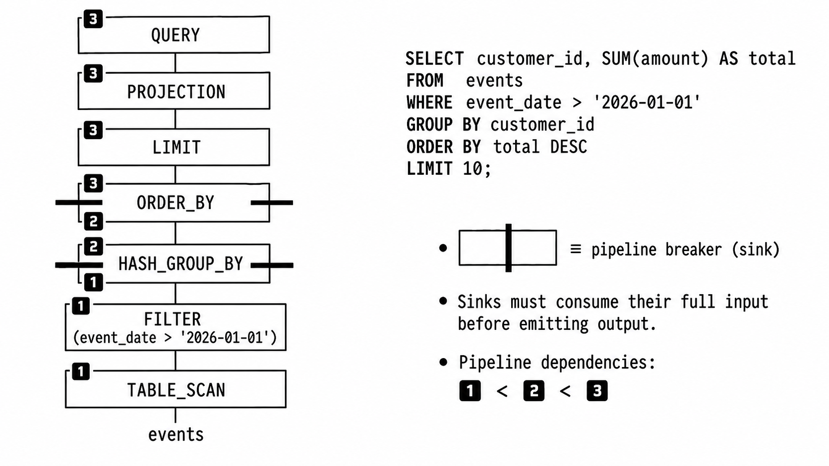
Going back to our original query, the physical plan may look something like this:回到最初的查询，物理计划可能如下所示：

• Pipeline 1: ends at the GROUP BY sink:
  scan events → filter event_date > '2026-01-01' → write into GROUP BY's hash table管道 1：在 GROUP BY sink 结束：扫描 events → 过滤 event_date > '2026-01-01' → 写入 GROUP BY 的哈希表
• Pipeline 2: ends at the ORDER BY sink:
  read groups out of the hash table → write them into the sorted run管道 2：在 ORDER BY sink 结束：从哈希表读取分组 → 写入已排序的运行
• Pipeline 3: the final assembly line:
  read sorted runs → take the first 10 rows → return results管道 3：最终装配线：读取已排序的运行 → 取前 10 行 → 返回结果

Each pipeline runs in parallel internally. Multiple threads run the entire assembly line at once, each on its own morsel of input. Pipelines that depend on each other run in sequence, because pipeline 2 can't start reading until pipeline 1's GROUP BY is done writing.每个管道内部并行运行。多个线程同时执行完整的装配线，各自处理自己的 morsel 输入。相互依赖的管道顺序执行，因为管道 2 必须等管道 1 的 GROUP BY 完成写入后才能开始读取。

What Happens in a Sink#Sink 中会发生什么#

A sink runs in three phases: sink, combine, and finalize. Sink 运行三个阶段：sink、combine 和 finalize。

Sink#Sink#

Every thread accepts chunks (DuckDB's 2048 row batches) and writes them into its own local state, for example, its own hash table for a HASH_GROUP_BY, its own sorted run for ORDER_BY, its own partial aggregate for UNGROUPED_AGGREGATE, its own hash table for the build side of HASH_JOIN. Threads do not share state. If every thread wrote into one shared hash table, they'd be fighting for a lock on every insert. Local state lets each thread sink at full speed with no coordination.每个线程接受块（DuckDB 的 2048 行批次），并写入自己的本地状态，例如 HASH_GROUP_BY 的本地哈希表、ORDER_BY 的本地已排序运行、UNGROUPED_AGGREGATE 的本地部分聚合、HASH_JOIN 构建端的本地哈希表。线程之间不共享状态。如果所有线程写入同一个共享哈希表，它们将在每次插入时争夺锁。本地状态让每个线程能够全速 sink 而无需协调。

Combine#Combine#

Once every thread finishes writing to its local space, the results have to merge into a single global state. For a GROUP BY, that means combining the partial sums and counts for each group across all the thread-local hash tables. DuckDB designs the sink so the combine step itself runs across all cores, rather than as a single-threaded merge at the end (covered in Part 3).当所有线程完成对本地空间的写入后，需要把结果合并为单一的全局状态。对于 GROUP BY，这意味着把所有线程本地哈希表中每个分组的部分求和与计数合并。DuckDB 设计的 sink 使得 combine 步骤本身也在所有核心上并行运行，而不是在最后进行单线程合并（第 3 部分会详细介绍）。

Finalize#Finalize#

The merged global state is read out as the input to the next pipeline. For our GROUP BY, that'll be a stream of customer_id, total) rows.合并后的全局状态作为下一个管道的输入被读取。对于我们的 GROUP BY，这将是一系列 `(customer_id, total)` 行。

Parallelism is Local#并行性是本地的#

A pipeline runs across all cores by giving each thread its own morsel of input. A sink runs across all cores by giving each thread its own local state and merging in parallel. DuckDB does not try to plan global parallelism for the whole query, it parallelizes one pipeline at a time. This is a part of what makes morsel-driven parallelism (covered in Part 3) and vectorized execution (covered in Part 2) work.一个管道通过为每个线程分配自己的 morsel 输入来跨所有核心运行。一个 sink 通过为每个线程提供本地状态并并行合并来跨所有核心运行。DuckDB 并不尝试为整个查询规划全局并行，而是一次并行化一个管道。这是 morsel‑驱动并行（第 3 部分）和向量化执行（第 2 部分）能够发挥作用的原因之一。

The Storage Layer#存储层#

The amazing thing about DuckDB is that it can turn most files into a SQL database, and in fact is often used to directly query file formats like Parquet, CSV, JSON, XLSX, etc.DuckDB 的惊人之处在于它可以把大多数文件直接当作 SQL 数据库使用，事实上它经常被用于直接查询 Parquet、CSV、JSON、XLSX 等文件格式。

DuckDB database#DuckDB 数据库#

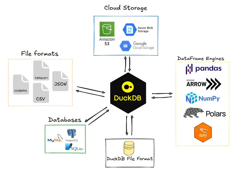
A DuckDB database is a single file, conventionally .duckdb or .db. This was inspired by SQLite. One file is easy to move, backup, and share.DuckDB 数据库是单个文件，通常以 .duckdb 或 .db 为后缀。这一设计受 SQLite 启发。单文件易于移动、备份和共享。

Inside the file, data is broken into fixed-size blocks. The default block size is 256 KB, though smaller block sizes (down to 16 KB) can be configured. The headers contain metadata like magic bytes, storage format versions, database headers, etc. 在文件内部，数据被划分为固定大小的块。默认块大小为 256 KB，虽然可以配置更小的块（最小 16 KB）。头部包含元数据，如魔术字节、存储格式版本、数据库头等。

Every block also carries a checksum, a small value computed from the block's contents. When DuckDB reads a block, it recomputes the checksum and compares. If the values don't match, the data has been corrupted somehow, and DuckDB raises an error. Checksums are important because bits occasionally flip in memory or on disk: a cosmic ray hits a cell, a firmware bug drops a byte, a flaky cable corrupts a write, etc. Cloud data warehouses can mitigate this with built-in error correction in memory and redundancy across disks. Consumer hardware like laptops or edge devices generally have less protection, so checksumming is a useful backstop.每个块还携带校验和，这是根据块内容计算的一个小值。当 DuckDB 读取块时，会重新计算校验和并进行比较。如果不匹配，说明数据已损坏，DuckDB 将抛出错误。校验和很重要，因为内存或磁盘上偶尔会出现位翻转：宇宙射线击中单元格、固件错误导致字节丢失、线缆不稳导致写入损坏等。云数据仓库可以通过内存错误纠正和磁盘冗余来缓解这些问题。普通笔记本或边缘设备的保护较少，校验和因此成为有用的后备。

Columns, row groups, zone maps#列、行组、分区映射#

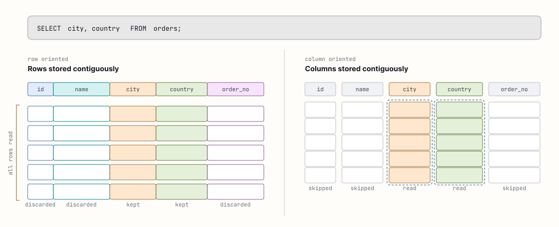
Inside the blocks, columns are stored separately from each other. A row store keeps entire records contiguous on disk. For example:在块内部，列是相互独立存储的。行存储则把整条记录连续存放在磁盘上。例如：

[id_1, name_1, age_1]
[id_2, name_2, age_2]
[id_3, name_3, age_3]

This is fast for queries like SELECT * FROM users WHERE id = 42, because the record's bytes sit close together physically in memory.这对于 `SELECT * FROM users WHERE id = 42` 之类的查询很快，因为记录的字节在内存中物理上相邻。

Column stores keep columns contiguous on disk.列式存储则把列在磁盘上连续存放。

[id_1, id_2, id_3]
[name_1, name_2, name_3]
[age_1, age_2, age_3]

A query that reads 4 columns from a 300 column table only needs to read those 4 columns. On a row store, all 300 columns would be read and 296 of those will need to be discarded. This is why organizations use column stores (Snowflake, BigQuery, ClickHouse, etc.) for analytics: queries tend to be selective, group on, and aggregate a few columns.查询只读取 300 列表中 4 列时，只需读取这 4 列。行存储则会读取全部 300 列，其中 296 列需要被丢弃。这就是组织使用列式存储（Snowflake、BigQuery、ClickHouse 等）进行分析的原因：查询往往只涉及少量列的过滤、分组和聚合。

Row Groups#行组#

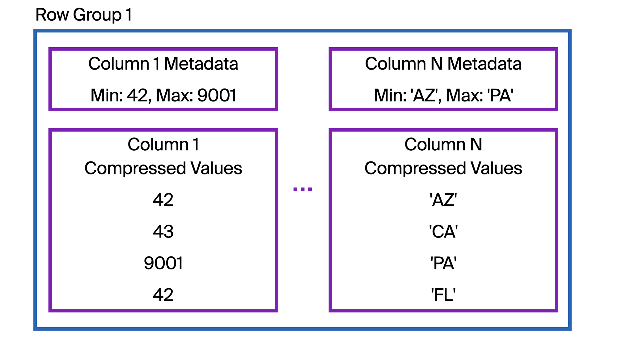
Each column is split into row groups of up to 122,880 rows, and within a row group, into column segments that typically map to a single 256 KB block. A row group is a unit of parallelism. A query running on 8 threads should have at least 8 row groups in scope to keep every thread busy.每列被划分为最多 122,880 行的行组，在行组内部进一步划分为通常映射到单个 256 KB 块的列段。行组是并行度的单位。使用 8 线程运行的查询应当至少有 8 个行组在范围内，以保持每个线程都有工作。

Zone Maps#分区映射（Zone Maps）#

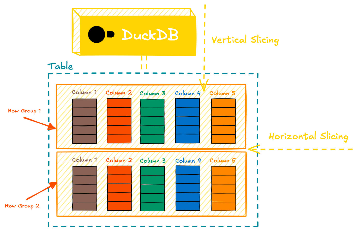
Each row group also carries a zone map. A zone map contains the min and max values in a row group, plus a null count. When a scan runs with a predicate like WHERE event_date > '2026-01-01', DuckDB checks each row group's max value before reading in any of its data. Row groups whose max event_date is on or before '2026-01-01' are skipped entirely.每个行组还携带一个分区映射。分区映射包含该行组的最小值、最大值以及空值计数。当使用类似 `WHERE event_date > '2026-01-01'` 的谓词进行扫描时，DuckDB 会在读取任何数据之前检查每个行组的最大值。最大值在 `'2026-01-01'` 之前或等于该日期的行组会被完全跳过。

This a similar technique major cloud data warehouses use, just under different names. Snowflake calls it micro-partition pruning, BigQuery calls it block pruning, ClickHouse uses minmax data skipping indexes.这与主要云数据仓库使用的技术类似，只是名称不同。Snowflake 称之为 micro‑partition pruning，BigQuery 称之为 block pruning，ClickHouse 使用 min‑max 数据跳过索引。

Zone map effectiveness depends heavily on column ordering. A column that's sorted or naturally ordered by an insert timestamp gives narrow min-max spans per row group. A column whose values are scattered randomly across the table gives spans that cover wide ranges, and the zonemap is much less effective.分区映射的效果高度依赖列的排序。按插入时间戳排序或自然有序的列在每个行组内的 min‑max 范围很窄。相反，值随机分布的列会产生宽范围的 span，分区映射的效果大打折扣。

Parquet#Parquet#

Most of the time, practitioners aren't querying DuckDB tables. They're pointing DuckDB at Parquet files. There are two common patterns:大多数情况下，使用者并不是查询 DuckDB 表，而是把 DuckDB 指向 Parquet 文件。有两种常见模式：

-- Query a parquet file directly
SELECT
  customer_id
  , SUM(amount) as total_amount
FROM read_parquet('/my/nice/files/*.parquet', union_by_name=TRUE)
WHERE
  event_date > '2026-01-01'
GROUP BY ALL;

-- Or load it into a DuckDB table first
CREATE TABLE events AS
SELECT * FROM read_parquet('s3://bucket/events/*.parquet');

Why is querying Parquet files so fast? DuckDB hasn't converted the data into its own format. There's no zone map built by DuckDB, no DuckDB-side compression, no .duckdb file. And yet, some queries run roughly as fast as a native DuckDB table.为什么查询 Parquet 文件如此快速？DuckDB 并没有把数据转换为自己的格式。没有 DuckDB 构建的分区映射、没有 DuckDB 侧压缩、也没有 .duckdb 文件。然而，一些查询的速度几乎与本地 DuckDB 表相当。

Parquet has similar design principles as DuckDB's native format:Parquet 与 DuckDB 原生格式有相似的设计原则：

• Parquet is columnar. Each column lives in its own column chunk inside a row group. DuckDB reads only the column chunks the query references.Parquet 是列式的。每列在行组内部都有自己的列块。DuckDB 只读取查询涉及的列块。
• Parquet stores min/max statistics per row group per column. DuckDB uses those same statistics exactly the way it uses zone maps.Parquet 为每个行组的每列存储 min/max 统计信息。DuckDB 正好使用这些统计信息，就像使用分区映射一样。

When querying Parquet, DuckDB reads the footer to discover the file's schema and row group statistics. It uses those statistics to determine which row groups can satisfy query predicates. For each surviving row group, it reads only the column chunks the query needs, decompresses them, and feeds them into the pipeline-and-sink we described earlier.查询 Parquet 时，DuckDB 读取文件尾部以获取模式和行组统计信息。它利用这些统计信息决定哪些行组能够满足查询谓词。对于每个保留下来的行组，只读取查询需要的列块，解压后送入前文描述的管道‑sink。

When a file is stored remotely, DuckDB doesn't download the whole file. It issues an HTTP request to fetch just the footer, decides which row groups and column chunks it needs, then issues requests to fetch only those bytes. A WHERE clause that prunes properly can dramatically increase performance over the wire.当文件存储在远程时，DuckDB 并不会下载整个文件。它先发起 HTTP 请求仅获取尾部，决定需要哪些行组和列块，然后只请求这些字节。有效的 WHERE 子句裁剪可以显著提升跨网络的性能。

CSVs#CSV#

CSV is the opposite of Parquet, it's not self-describing. Parquet effectively hands DuckDB a schema, statistics, chunked columns with compressed data. CSVs don't. They're just text. DuckDB needs to figure out what character separates columns, are values quoted, how are quotes escaped, does the first row contain column names, and what type each column should be. DuckDB does this with its CSV sniffer.CSV 与 Parquet 相反，它不是自描述的。Parquet 为 DuckDB 提供了模式、统计信息、分块列和压缩数据，而 CSV 只是文本。DuckDB 必须判断列分隔符是什么、值是否被引号包裹、引号如何转义、首行是否包含列名以及每列的类型。DuckDB 使用 CSV sniffing（嗅探）来完成这些工作。

SELECT *
FROM 'events.csv';

-- Alternatively
SELECT *
FROM read_csv('events.csv');

When DuckDB reads a CSV, it automatically tries to detect three main things: the dialect, the column types, and whether the file has a header row.当 DuckDB 读取 CSV 时，它会自动尝试检测三件主要内容：方言、列类型以及文件是否有标题行。

Dialect Detection#方言检测#

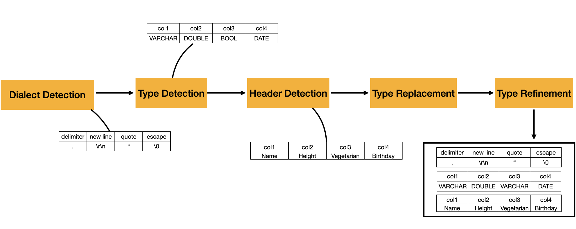
The dialect is the file’s parsing grammar: delimiter, quote character, escape character, and newline style. DuckDB tests candidate dialects and chooses the one that produces the most consistent rows and the highest number of columns. For example, a file like this:方言是文件的解析语法：分隔符、引号字符、转义字符和换行风格。DuckDB 会测试候选方言并选择产生最一致行数且列数最多的那一个。例如，下面这样的文件：

Company|Category|City|IsSuperCool
DuckDB|OLAP database|Amsterdam, Netherlands|True
Snowflake|data warehouse|Bozeman, MT|True
BigQuery|data warehouse|Mountain View, CA|N/A
Greybeam|multi-engine router|San Francisco, CA|True

Should be split on |, not ,, even though the city names contain commas. The sniffer can figure that out because | produces a consistent four-column table.应该使用 `|` 进行分割，而不是 `,`，即使城市名称中包含逗号。嗅探器能够判断出来，因为 `|` 能产生一致的四列表。

Column Types#列类型#

After the dialect is chosen, DuckDB detects column types by trying to convert sampled values in each column to candidate types. If a value cannot be converted to a candidate type, that type is removed from the candidate set for that column. After the samples are processed, DuckDB chooses the remaining candidate type with the highest priority. The documented default candidate types, in priority order, are NULL, BOOLEAN, TIME, DATE, TIMESTAMP, TIMESTAMPTZ, BIGINT, DOUBLE, and VARCHAR. Since every value can be represented as VARCHAR, it is the fallback type.在选择方言后，DuckDB 通过尝试将每列的抽样值转换为候选类型来检测列类型。如果某个值无法转换为某个候选类型，则该类型会从该列的候选集合中移除。处理完抽样后，DuckDB 会选择剩余候选类型中优先级最高的。文档中默认的候选类型按优先级顺序为 NULL、BOOLEAN、TIME、DATE、TIMESTAMP、TIMESTAMPTZ、BIGINT、DOUBLE 和 VARCHAR。由于每个值都可以表示为 VARCHAR，它是回退类型。

Headers#标题#

Header detection comes next. If the first row looks different from the rows below it, for example, strings like Company and Category are treated as the column names. Otherwise it generates default names like column0, column1, etc.接下来进行标题检测。如果第一行看起来与下面的行不同，例如字符串 "Company" 和 "Category" 被视为列名。否则会生成默认名称，如 column0、column1 等。

The sniffer works from a sample rather than scanning the full file. The default sample size is 20,480 rows. You can increase this, or set sample_size = -1 to inspect the whole file.嗅探器是基于抽样而不是扫描整个文件工作。默认抽样大小为 20,480 行。您可以增大此值，或将 sample_size 设置为 -1 以检查整个文件。

Execution#执行#

Clearly a lot of work happens before a query actually runs. It gets parsed into an AST, bound to the schema, optimized through ~30 passes, and compiled into a physical plan. Even the storage layer does so much work in advance.显然在查询实际运行之前已经做了大量工作。查询会被解析为 AST，绑定到模式，经过约 30 次优化传递，并编译成物理计划。甚至存储层也会提前完成大量工作。

Part 2 picks up at execution. Stay tuned!第 2 部分从执行开始。敬请期待！

At Greybeam, this is part of why building a multi-engine router is so exciting for the future of data. It's clear that DuckDB is fast. DuckDB's strengths are real. So are Snowflake's. So are BigQuery's. 在 Greybeam，这也是构建多引擎路由器对数据未来如此令人兴奋的原因之一。显而易见，DuckDB 很快。DuckDB 的优势是真实的，Snowflake 的优势也是如此，BigQuery 的优势也是如此。

We believe in a future where data teams can use the query engine built to run each query the fastest. Come along for the ride.我们相信未来数据团队能够使用为每个查询提供最快运行速度的查询引擎。一起加入这段旅程吧。