A Visual Guide to Quantization量化视觉指南

Demystifying the Compression of Large Language Models揭秘大语言模型压缩技术

Translations - Korean - Chinese - French翻译 - 韩语 - 中文 - 法语

As their name suggests, Large Language Models (LLMs) are often too large to run on consumer hardware. These models may exceed billions of parameters and generally need GPUs with large amounts of VRAM to speed up inference.顾名思义，大语言模型（LLM）通常体积庞大，难以在消费级硬件上运行。这些模型可能拥有数十亿个参数，通常需要配备大容量显存（VRAM）的 GPU 来加速推理。

As such, more and more research has been focused on making these models smaller through improved training, adapters, etc. One major technique in this field is called quantization.因此，越来越多的研究致力于通过改进训练、适配器（adapter）等技术来缩小模型体积。该领域的一项主要技术被称为“量化”。

In this post, I will introduce the field of quantization in the context of language modeling and explore concepts one by one to develop an intuition about the field. We will explore various methodologies, use cases, and the principles behind quantization. 在本文中，我将介绍语言模型背景下的量化领域，并逐一探讨相关概念，以帮助大家建立对该领域的直观理解。我们将探索各种方法论、应用场景以及量化背后的原理。

In this visual guide, there are more than 50 custom visuals to help you develop an intuition about quantization!本视觉指南包含 50 多张自定义图表，旨在帮助您直观地理解量化！

To see more visualizations related to LLMs and to support this newsletter, check out the book I wrote on Large Language Models!想要查看更多与大语言模型相关的可视化内容并支持本通讯，请查看我撰写的大语言模型书籍！

Official website of the book. You can order the book on Amazon. All code is uploaded to GitHub.书籍官方网站。您可以在亚马逊上订购本书。所有代码均已上传至 GitHub。

P.S. If you read the book, a quick review would mean the world—it really helps us authors! 附：如果您读过这本书，写一段简短的书评对我意义重大——这对我们作者非常有帮助！

Part 1: The “Problem“ with LLMs

第一部分：大语言模型的“问题”

LLMs get their name due to the number of parameters they contain. Nowadays, these models typically have billions of parameters (mostly weights) which can be quite expensive to store. 大语言模型之所以得名，是因为它们包含大量的参数。如今，这些模型通常拥有数十亿个参数（主要是权重），存储成本相当高昂。

During inference, activations are created as a product of the input and the weights, which similarly can be quite large.在推理过程中，激活值（activations）由输入与权重的乘积产生，同样可能非常庞大。

As a result, we would like to represent billions of values as efficiently as possible, minimizing the amount of space we need to store a given value.因此，我们希望尽可能高效地表示这数十亿个数值，从而最大限度地减少存储给定数值所需的空间。

Let’s start from the beginning and explore how numerical values are represented in the first place before optimizing them. 让我们从基础开始，在进行优化之前，先探讨数值最初是如何表示的。

How to Represent Numerical Values

如何表示数值

A given value is often represented as a floating point number (or floats in computer science): a positive or negative number with a decimal point. 给定的数值通常表示为浮点数（计算机科学中的 float）：即带有小数点的正数或负数。

These values are represented by “bits”, or binary digits. The IEEE-754 standard describes how bits can represent one of three functions to represent the value: the sign, exponent, or fraction (or mantissa).这些数值由“位”（bit，二进制数字）表示。IEEE-754 标准描述了位如何通过符号、指数和分数（或尾数）这三个部分来表示数值。

Together, these three aspects can be used to calculate a value given a certain set of bit values:这三个部分共同作用，可以根据一组给定的位值计算出数值：

The more bits we use to represent a value, the more precise it generally is:通常情况下，用于表示数值的位数越多，精度就越高：

Memory Constraints

内存限制

The more bits we have available, the larger the range of values that can be represented.可用的位数越多，能表示的数值范围就越大。

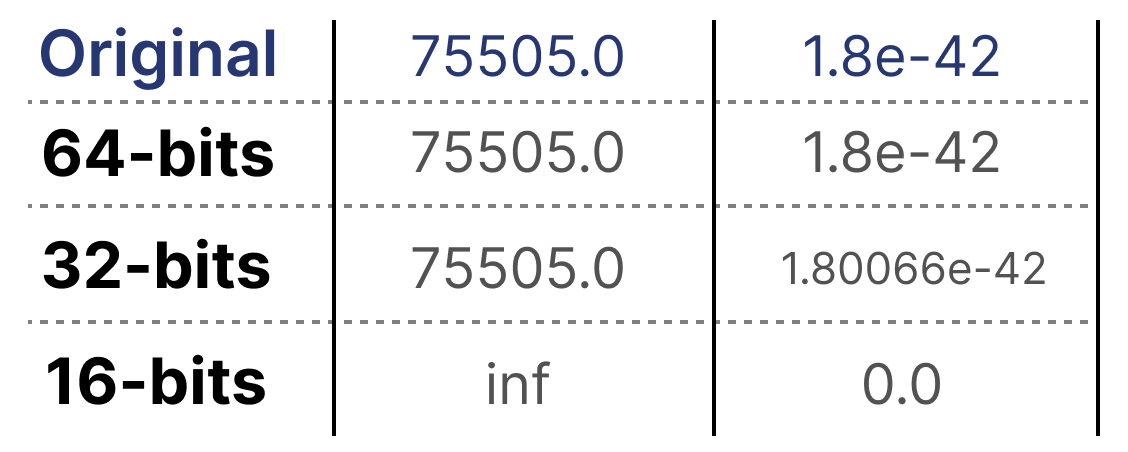
The interval of representable numbers a given representation can take is called the dynamic range whereas the distance between two neighboring values is called precision.给定表示法所能涵盖的可表示数值区间称为“动态范围”，而两个相邻数值之间的距离称为“精度”。

A nifty feature of these bits is that we can calculate how much memory your device needs to store a given value. Since there are 8 bits in a byte of memory, we can create a basic formula for most forms of floating point representation.位的一个巧妙之处在于，我们可以计算设备存储给定数值所需的内存大小。由于 1 字节内存包含 8 位，我们可以为大多数浮点表示形式建立一个基本公式。

NOTE: In practice, more things relate to the amount of (V)RAM you need during inference, like the context size and architecture.注意：在实践中，推理过程中所需的显存（VRAM）量还与上下文长度和架构等其他因素有关。

Now let’s assume that we have a model with 70 billion parameters. Most models are natively represented with float 32-bit (often called full-precision), which would require 280GB of memory just to load the model.现在假设我们有一个拥有 700 亿参数的模型。大多数模型原生使用 32 位浮点数（通常称为全精度）表示，仅加载模型就需要 280GB 的内存。

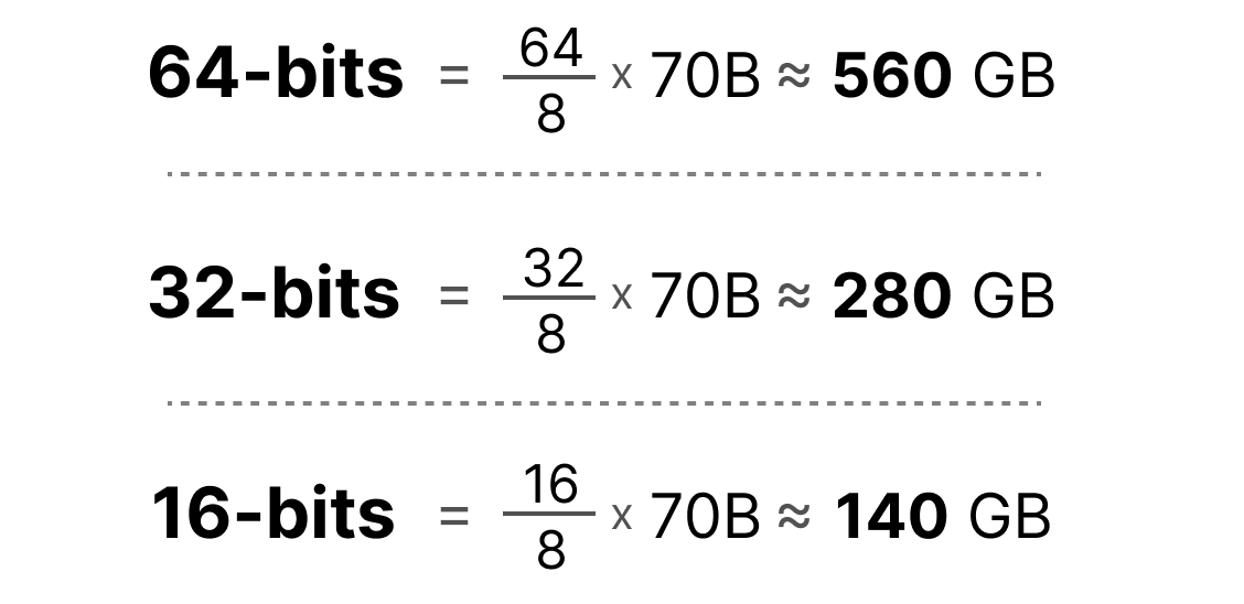
As such, it is very compelling to minimize the number of bits to represent the parameters of your model (as well as during training!). However, as the precision decreases the accuracy of the models generally does as well. 因此，最大限度地减少表示模型参数所需的位数（以及训练期间的位数！）非常有必要。然而，随着精度的降低，模型的准确性通常也会下降。

We want to reduce the number of bits representing values while maintaining accuracy… This is where quantization comes in!我们希望在保持准确性的同时减少表示数值的位数……这就是量化的用武之地！

Part 2: Introduction to Quantization

第二部分：量化简介

Quantization aims to reduce the precision of a model’s parameter from higher bit-widths (like 32-bit floating point) to lower bit-widths (like 8-bit integers).量化的目的是将模型参数的精度从高位宽（如 32 位浮点数）降低到低位宽（如 8 位整数）。

There is often some loss of precision (granularity) when reducing the number of bits to represent the original parameters. 在减少表示原始参数的位数时，通常会损失一定的精度（粒度）。

To illustrate this effect, we can take any image and use only 8 colors to represent it:为了说明这种效果，我们可以取任意一张图片，仅使用 8 种颜色来呈现它：

Image adapted from the original by Slava Sidorov.图片改编自 Slava Sidorov 的原图。

Notice how the zoomed-in part seems more “grainy” than the original since we can use fewer colors to represent it.请注意，放大后的部分看起来比原图更“粗糙”，因为我们使用的颜色变少了。

The main goal of quantization is to reduce the number of bits (colors) needed to represent the original parameters while preserving the precision of the original parameters as best as possible. 量化的主要目标是在尽可能保留原始参数精度的同时，减少表示它们所需的位数（颜色）。

Common Data Types

常见数据类型

First, let’s look at common data types and the impact of using them rather than 32-bit (called full-precision or FP32) representations.首先，让我们看看常见的数据类型，以及使用它们而非 32 位（全精度或 FP32）表示所带来的影响。

FP16

Let’s look at an example of going from 32-bit to 16-bit (called half precision or FP16) floating point:让我们看一个从 32 位浮点数转换为 16 位（半精度或 FP16）浮点数的例子：

Notice how the range of values FP16 can take is quite a bit smaller than FP32. 请注意，FP16 所能涵盖的数值范围比 FP32 小得多。

BF16

To get a similar range of values as the original FP32, bfloat 16 was introduced as a type of “truncated FP32”:为了获得与原始 FP32 相似的数值范围，bfloat16 被引入，作为一种“截断后的 FP32”类型：

BF16 uses the same amount of bits as FP16 but can take a wider range of values and is often used in deep learning applications. BF16 使用的位数与 FP16 相同，但可以涵盖更广的数值范围，常用于深度学习应用。

INT8

When we reduce the number of bits even further, we approach the realm of integer-based representations rather than floating-point representations. To illustrate, going FP32 to INT8, which has only 8 bits, results in a fourth of the original number of bits:当我们进一步减少位数时，就会进入基于整数的表示领域，而非浮点表示。举例来说，从 FP32 转换为仅有 8 位的 INT8，位数为原来的四分之一：

Depending on the hardware, integer-based calculations might be faster than floating-point calculations but this isn’t always the case. However, computations are generally faster when using fewer bits. 根据硬件的不同，基于整数的计算可能比浮点计算更快，但并非总是如此。不过，使用较少的位数通常能加快计算速度。

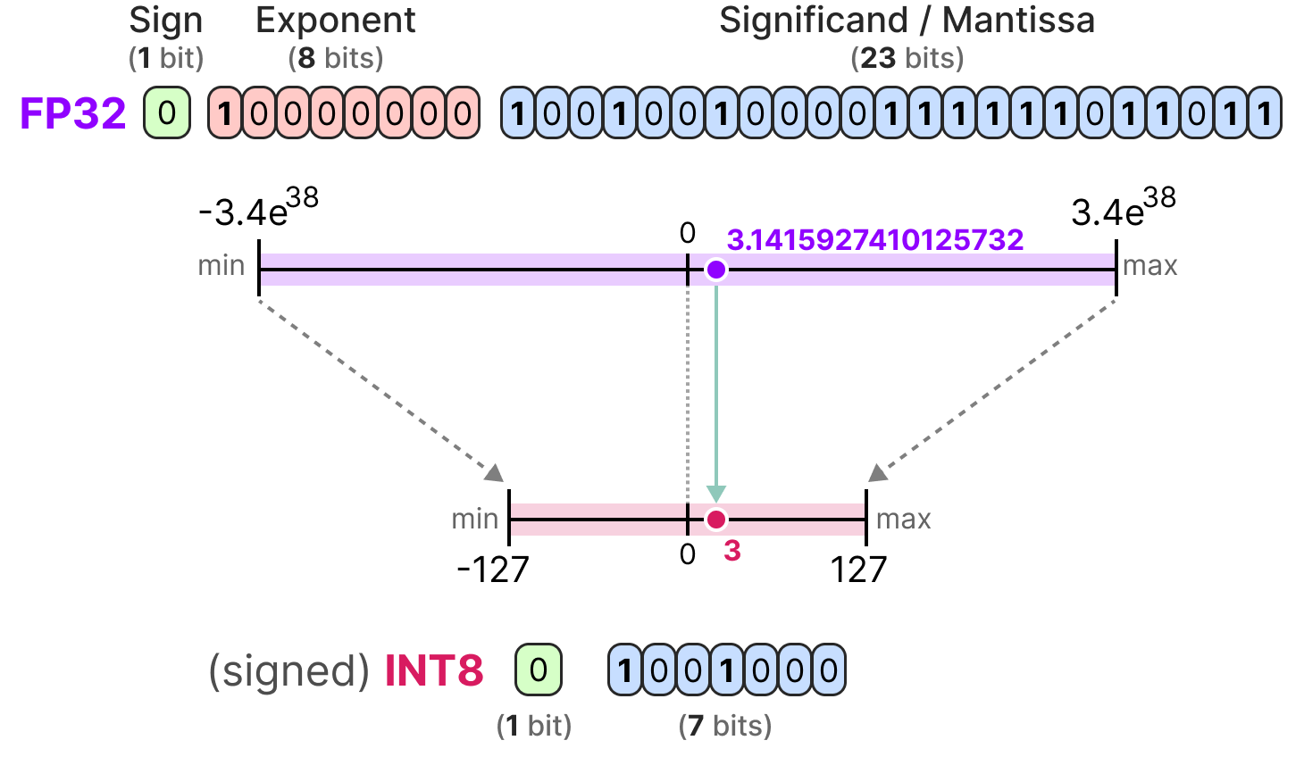
For each reduction in bits, a mapping is performed to “squeeze” the initial FP32 representations into lower bits. 对于每一次位数的减少，都会执行一次映射，将初始的 FP32 表示“压缩”到更低的位数中。

In practice, we do not need to map the entire FP32 range [-3.4e38, 3.4e38] into INT8. We merely need to find a way to map the range of our data (the model’s parameters) into INT8. 在实践中，我们不需要将整个 FP32 范围 [-3.4e38, 3.4e38] 映射到 INT8。我们只需要找到一种方法，将数据（模型参数）的范围映射到 INT8 即可。

Common squeezing/mapping methods are symmetric and asymmetric quantization and are forms of linear mapping. 常见的压缩/映射方法包括对称量化和非对称量化，它们都是线性映射的形式。

Let’s explore these methods to quantize from FP32 to INT8.让我们探讨这些将 FP32 量化为 INT8 的方法。

Symmetric Quantization

对称量化

In symmetric quantization, the range of the original floating-point values is mapped to a symmetric range around zero in the quantized space. In the previous examples, notice how the ranges before and after quantization remain centered around zero.在对称量化中，原始浮点值的范围被映射到量化空间中以零为中心的对称范围内。在之前的例子中，请注意量化前后的范围是如何保持以零为中心的。

This means that the quantized value for zero in the floating-point space is exactly zero in the quantized space.这意味着浮点空间中的零在量化空间中对应的量化值恰好也是零。

A nice example of a form of symmetric quantization is called absolute maximum (absmax) quantization. 对称量化的一种常用示例称为绝对最大值（absmax）量化。

Given a list of values, we take the highest absolute value (α) as the range to perform the linear mapping.给定一系列数值，我们取绝对值最大的数（α）作为执行线性映射的范围。

Note the [-127, 127] range of values represents the restricted range. The unrestricted range is [-128, 127] and depends on the quantization method.注意，[-127, 127] 的数值范围代表受限范围。非受限范围是 [-128, 127]，具体取决于量化方法。

Since it is a linear mapping centered around zero, the formula is straightforward. 由于这是一个以零为中心的线性映射，其公式非常直观。

We first calculate a scale factor (s) using:我们首先计算比例因子（s）：

• b is the number of bytes that we want to quantize to (8), b 是我们想要量化到的字节数（8），

• α is the highest absolute value, α 是绝对值最大的数，

Then, we use the s to quantize the input x:然后，我们使用 s 来量化输入 x：

Filling in the values would then give us the following:代入这些值，我们得到：

To retrieve the original FP32 values, we can use the previously calculated scaling factor (s) to dequantize the quantized values.要恢复原始的 FP32 数值，我们可以使用之前计算出的比例因子（s）对量化值进行反量化。

Applying the quantization and then dequantization process to retrieve the original looks as follows:应用量化然后反量化以恢复原始值的过程如下：

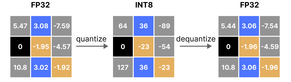
You can see certain values, such as 3.08 and 3.02 being assigned to the INT8, namely 36. When you dequantize the values to return to FP32, they lose some precision and are not distinguishable anymore. 可以看到某些数值（如 3.08 和 3.02）被分配到了同一个 INT8 值，即 36。当您反量化这些数值回到 FP32 时，它们丢失了一些精度，变得无法区分。

This is often referred to as the quantization error which we can calculate by finding the difference between the original and dequantized values.这通常被称为量化误差，我们可以通过计算原始值与反量化值之间的差值来得出。

Generally, the lower the number of bits, the more quantization error we tend to have.通常，位数越低，量化误差往往越大。

Asymmetric Quantization

非对称量化

Asymmetric quantization, in contrast, is not symmetric around zero. Instead, it maps the minimum (β) and maximum (α) values from the float range to the minimum and maximum values of the quantized range. 相比之下，非对称量化并不以零为中心。相反，它将浮点范围内的最小值（β）和最大值（α）映射到量化范围的最小值和最大值。

The method we are going to explore is called zero-point quantization.我们将要探讨的方法称为零点量化（zero-point quantization）。

Notice how the 0 has shifted positions? That’s why it’s called asymmetric quantization. The min/max values have different distances to 0 in the range [-7.59, 10.8].注意到 0 的位置发生了偏移吗？这就是它被称为非对称量化的原因。在范围 [-7.59, 10.8] 中，最小值和最大值到 0 的距离各不相同。

Due to its shifted position, we have to calculate the zero-point for the INT8 range to perform the linear mapping. As before, we also have to calculate a scale factor (s) but use the difference of INT8’s range instead [-128, 127]由于其位置发生了偏移，我们必须计算 INT8 范围内的零点以执行线性映射。和之前一样，我们还需要计算比例因子（s），但使用的是 INT8 范围 [-128, 127] 的差值。

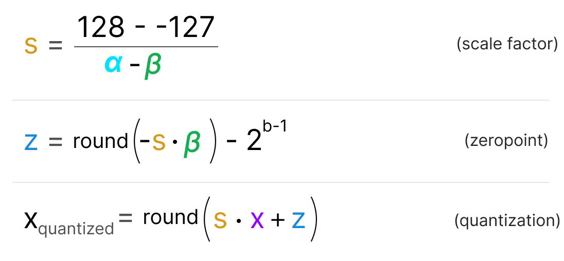
Notice how this is a bit more involved due to the need to calculate the zeropoint (z) in the INT8 range to shift the weights.请注意，由于需要计算 INT8 范围内的零点（z）来平移权重，这个过程稍微复杂一些。

As before, let’s fill in the formula:和之前一样，让我们代入公式：

To dequantize the quantized from INT8 back to FP32, we will need to use the previously calculated scale factor (s) and zeropoint (z).要将量化后的 INT8 值反量化回 FP32，我们需要使用之前计算出的比例因子（s）和零点（z）。

Other than that, dequantization is straightforward:除此之外，反量化过程非常简单：

When we put symmetric and asymmetric quantization side-by-side, we can quickly see the difference between methods:当我们把对称量化和非对称量化放在一起比较时，可以很快看出两者的区别：

Note the zero-centered nature of symmetric quantization versus the offset of asymmetric quantization.请注意对称量化的零中心特性与非对称量化的偏移特性。

Range Mapping and Clipping

范围映射与裁剪

In our previous examples, we explored how the range of values in a given vector could be mapped to a lower-bit representation. Although this allows for the full range of vector values to be mapped, it comes with a major downside, namely outliers.在之前的例子中，我们探讨了如何将给定向量中的数值范围映射到低位表示。尽管这允许向量中的全部数值范围被映射，但它有一个主要的缺点，即异常值（outliers）。

Imagine that you have a vector with the following values:想象一下，您有一个包含以下数值的向量：

Note how one value is much larger than all others and could be considered an outlier. If we were to map the full range of this vector, all small values would get mapped to the same lower-bit representation and lose their differentiating factor:请注意，其中一个数值远大于其他所有数值，可以被视为异常值。如果我们映射该向量的全部范围，所有较小的数值都会被映射到相同的低位表示，从而失去它们的区分度：

This is the absmax method we used earlier. Note that the same behavior happens with asymmetric quantization if we do not apply clipping.这就是我们之前使用的 absmax 方法。请注意，如果不应用裁剪，非对称量化也会出现同样的情况。

Instead, we can choose to clip certain values. Clipping involves setting a different dynamic range of the original values such that all outliers get the same value.相反，我们可以选择裁剪某些数值。裁剪涉及设置原始数值的不同动态范围，使得所有异常值都获得相同的值。

In the example below, if we were to manually set the dynamic range to [-5, 5] all values outside that will either be mapped to -127 or to 127 regardless of their value:在下例中，如果我们手动将动态范围设置为 [-5, 5]，那么所有超出该范围的数值，无论其原值是多少，都将被映射为 -127 或 127：

The major advantage is that the quantization error of the non-outliers is reduced significantly. However, the quantization error of outliers increases.其主要优点是显著降低了非异常值的量化误差。然而，异常值的量化误差会增加。

Calibration

校准

In the example, I showed a naive method of choosing an arbitrary range of [-5, 5]. The process of selecting this range is known as calibration which aims to find a range that includes as many values as possible while minimizing the quantization error.在例子中，我展示了一种选择任意范围 [-5, 5] 的简单方法。选择该范围的过程称为“校准”，旨在找到一个既包含尽可能多数值，又能最大限度减小量化误差的范围。

Performing this calibration step is not equal for all types of parameters. 执行此校准步骤对于不同类型的参数并不相同。

Weights (and Biases)

权重（及偏置）

We can view the weights and biases of an LLM as static values since they are known before running the model. For instance, the ~20GB file of Llama 3 consists mostly of its weight and biases.我们可以将大语言模型的权重和偏置视为静态值，因为它们在运行模型之前就已经确定了。例如，Llama 3 的约 20GB 文件主要由其权重和偏置组成。

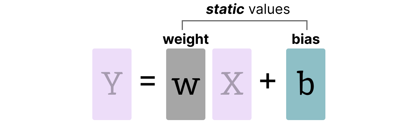
Since there are significantly fewer biases (millions) than weights (billions), the biases are often kept in higher precision (such as INT16), and the main effort of quantization is put towards the weights.由于偏置的数量（数百万）远少于权重（数十亿），偏置通常保持在较高精度（如 INT16），而量化的主要工作集中在权重上。

For weights, which are static and known, calibration techniques for choosing the range include:对于静态且已知的权重，选择范围的校准技术包括：

• Manually chosing a percentile of the input range手动选择输入范围的百分位数

• Optimize the mean squared error (MSE) between the original and quantized weights.优化原始权重与量化权重之间的均方误差（MSE）。

• Minimizing entropy (KL-divergence) between the original and quantized values最小化原始值与量化值之间的熵（KL 散度）

Choosing a percentile, for instance, would lead to similar clipping behavior as we have seen before.例如，选择百分位数会导致与我们之前看到的类似的裁剪行为。

Activations

激活值

The input that is continuously updated throughout the LLM is typically referred to as “activations”.在大语言模型中持续更新的输入通常被称为“激活值”。

Note that these values are called activations since they often go through some activation function, like sigmoid or relu.注意，这些值被称为激活值，因为它们通常会经过某些激活函数，如 sigmoid 或 relu。

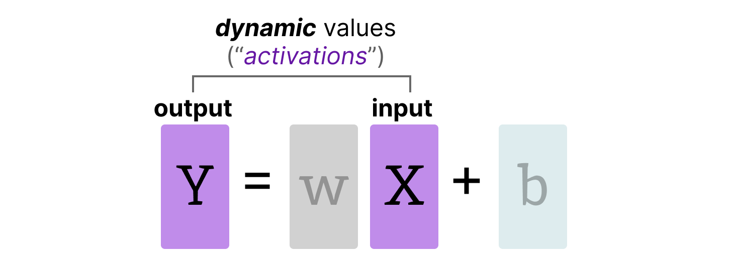
Unlike weights, activations vary with each input data fed into the model during inference, making it challenging to quantize them accurately. 与权重不同，激活值会随着推理过程中馈入模型的每个输入数据而变化，这使得准确量化它们具有挑战性。

Since these values are updated after each hidden layer, we only know what they will be during inference as the input data passes through the model.由于这些值在每一层隐藏层之后都会更新，我们只有在输入数据通过模型进行推理时，才能知道它们的值。

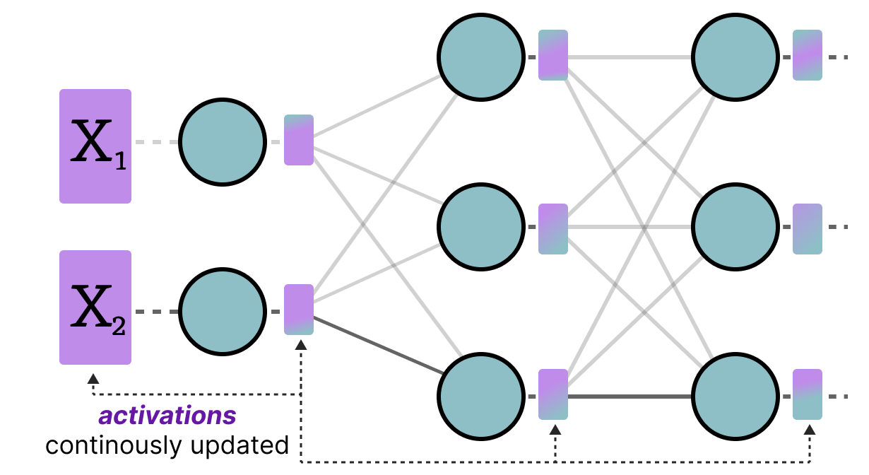
Broadly, there are two methods for calibrating the quantization method of the weights and activations:概括来说，有两种用于校准权重和激活值量化的方法：

• Post-Training Quantization (PTQ)训练后量化 (PTQ)

  • Quantization after training训练后的量化

• Quantization Aware Training (QAT)量化感知训练 (QAT)

  • Quantization during training/fine-tuning训练/微调期间的量化

Part 3: Post-Training Quantization

第三部分：训练后量化 (PTQ)

One of the most popular quantization techniques is post-training quantization (PTQ). It involves quantizing a model’s parameters (both weights and activations) after training the model. 最流行的量化技术之一是训练后量化 (PTQ)。它涉及在模型训练完成后对模型参数（权重和激活值）进行量化。

Quantization of the weights is performed using either symmetric or asymmetric quantization. 权重的量化使用对称或非对称量化来执行。

Quantization of the activations, however, requires inference of the model to get their potential distribution since we do not know their range.然而，激活值的量化需要对模型进行推理以获取其潜在分布，因为我们不知道它们的范围。

There are two forms of quantization of the activations:激活值的量化有两种形式：

• Dynamic Quantization动态量化

• Static Quantization静态量化

Dynamic Quantization

After data passes a hidden layer, its activations are collected:数据通过隐藏层后，收集其激活值：

This distribution of activations is then used to calculate the zeropoint (z) and scale factor (s) values needed to quantize the output:然后使用这些激活值的分布来计算量化输出所需的零点 (z) 和比例因子 (s)：

The process is repeated each time data passes through a new layer. Therefore, each layer has its own separate z and s values and therefore different quantization schemes.每次数据通过新层时，该过程都会重复。因此，每一层都有自己独立的 z 和 s 值，从而有不同的量化方案。

Static Quantization

In contrast to dynamic quantization, static quantization does not calculate the zeropoint (z) and scale factor (s) during inference but beforehand.与动态量化相反，静态量化不在推理过程中计算零点 (z) 和比例因子 (s)，而是提前计算。

To find those values, a calibration dataset is used and given to the model to collect these potential distributions.为了找到这些值，使用校准数据集馈入模型以收集这些潜在分布。

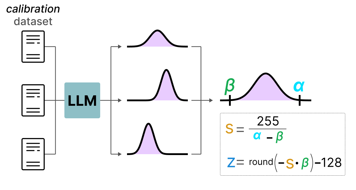
After these values have been collected, we can calculate the necessary s and z values to perform quantization during inference.收集这些值后，我们可以计算出在推理过程中执行量化所需的 s 和 z 值。

When you are performing actual inference, the s and z values are not recalculated but are used globally over all activations to quantize them.在实际执行推理时，s 和 z 值不会重新计算，而是全局应用于所有激活值以进行量化。

In general, dynamic quantization tends to be a bit more accurate since it only attempts to calculate the s and z values per hidden layer. However, it might increase compute time as these values need to be calculated.通常，动态量化往往更准确，因为它只尝试计算每层隐藏层的 s 和 z 值。然而，由于这些值需要计算，它可能会增加计算时间。

In contrast, static quantization is less accurate but is faster as it already knows the s and z values used for quantization.相比之下，静态量化精度较低，但速度更快，因为它已经预知了用于量化的 s 和 z 值。

The Realm of 4-bit Quantization

4 位量化的领域

Going below 8-bit quantization has proved to be a difficult task as the quantization error increases with each loss of bit. Fortunately, there are several smart ways to reduce the bits to 6, 4, and even 2-bits (although going lower than 4-bits using these methods is typically not advised). 事实证明，低于 8 位的量化是一项艰巨的任务，因为量化误差会随着位数的减少而增加。幸运的是，有几种巧妙的方法可以将位数减少到 6 位、4 位甚至 2 位（尽管通常不建议使用这些方法低于 4 位）。

We will explore two methods that are commonly shared on HuggingFace:我们将探讨两种在 HuggingFace 上常用的方法：

• GPTQ (full model on GPU)GPTQ（GPU 上的完整模型）

• GGUF (potentially offload layers on the CPU)GGUF（可将层卸载到 CPU 上）

GPTQ

GPTQ is arguably one of the most well-known methods used in practice for quantization to 4-bits.¹GPTQ 可以说是实践中用于 4 位量化的最著名方法之一。

It uses asymmetric quantization and does so layer by layer such that each layer is processed independently before continuing to the next:它使用非对称量化，并逐层进行，使得每一层在继续下一层之前都被独立处理：

During this layer-wise quantization process, it first converts the layer’s weights into the inverse-Hessian. It is a second-order derivative of the model’s loss function and tells us how sensitive the model's output is to changes in each weight.在这一层级的量化过程中，它首先将该层的权重转换为逆黑塞矩阵（inverse-Hessian）。它是模型损失函数的二阶导数，告诉我们模型的输出对每个权重的变化有多敏感。

Simplified, it essentially demonstrates the (inverse) importance of each weight in a layer.简单来说，它本质上展示了层中每个权重的（逆）重要性。

Weights associated with smaller values in the Hessian matrix are more crucial because small changes in these weights can lead to significant changes in the model's performance.黑塞矩阵中较小值所对应的权重更为关键，因为这些权重的微小变化可能导致模型性能的显著变化。

In the inverse-Hessian, lower values indicate more “important” weights.在逆黑塞矩阵中，较低的值表示更“重要”的权重。

Next, we quantize and then dequantize the weight of the first row in our weight matrix:接下来，我们对权重矩阵中第一行的权重进行量化和反量化：

This process allows us to calculate the quantization error (q) which we can weigh using the inverse-Hessian (h_1) that we calculated beforehand. 此过程允许我们计算量化误差 (q)，我们可以使用之前计算出的逆黑塞矩阵 (h_1) 对其进行加权。

Essentially, we are creating a weighted-quantization error based on the importance of the weight:本质上，我们正在根据权重的权重重要性创建一个加权量化误差：

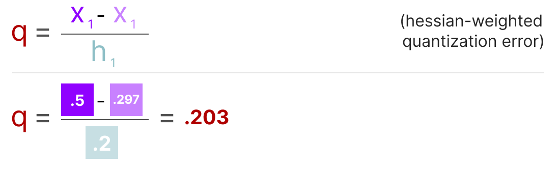
Next, we redistribute this weighted quantization error over the other weights in the row. This allows for maintaining the overall function and output of the network.接下来，我们将此加权量化误差重新分配到该行的其他权重上。这有助于保持网络的整体功能和输出。

For example, if we were to do this for the second weight, namely .3 (x_2), we would add the quantization error (q) multiplied by the inverse-Hessian of the second weight (h_2)例如，如果我们对第二个权重（即 .3 (x_2)）执行此操作，我们将加上量化误差 (q) 乘以第二个权重的逆黑塞矩阵 (h_2)。

We can do the same process over the third weight in the given row:我们可以在给定行的第三个权重上执行相同的过程：

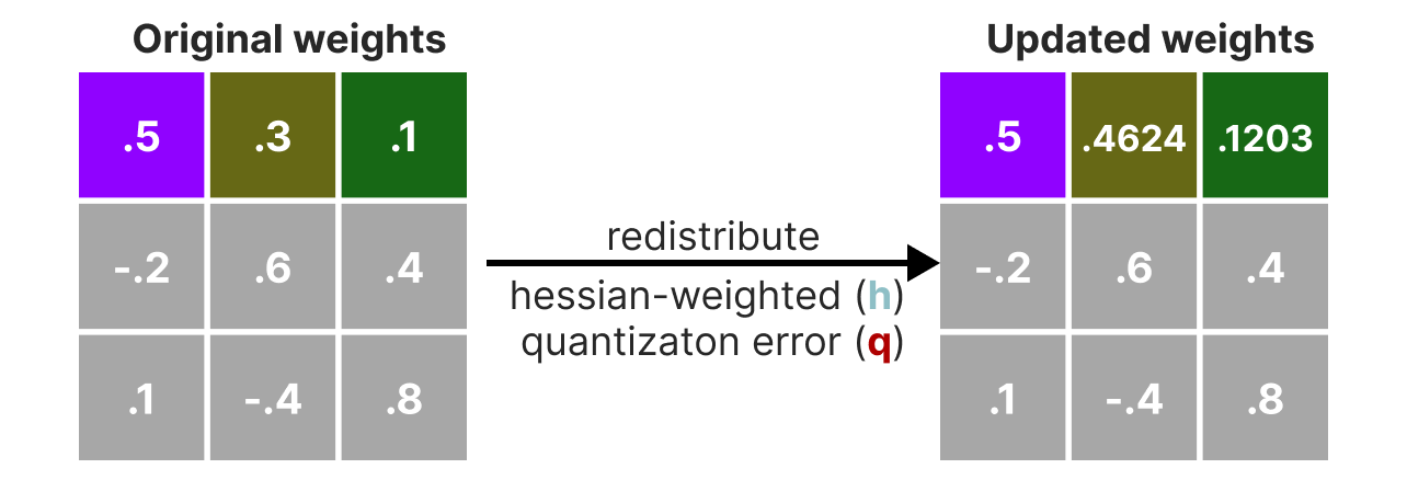
We iterate over this process of redistributing the weighted quantization error until all values are quantized.我们重复这个重新分配加权量化误差的过程，直到所有值都被量化。

This works so well because weights are typically related to one another. So when one weight has a quantization error, related weights are updated accordingly (through the inverse-Hessian).这种方法之所以效果显著，是因为权重通常彼此相关。因此，当一个权重出现量化误差时，相关的权重会相应地进行更新（通过逆黑塞矩阵）。

NOTE: The authors used several tricks to speed up computation and improve performance, such as adding a dampening factor to the Hessian, “lazy batching”, and precomputing information using the Cholesky method. I would highly advise checking out this YouTube video on the subject.注意：作者使用了多种技巧来加速计算和提高性能，例如在黑塞矩阵中添加阻尼因子、“惰性批处理”，以及使用 Cholesky 方法预计算信息。强烈建议观看关于此主题的 YouTube 视频。

TIP: Check out EXL2 if you want a quantization method aimed at performance optimizations and improving inference speed.提示：如果您想要一种旨在优化性能和提高推理速度的量化方法，请查看 EXL2。

GGUF

While GPTQ is a great quantization method to run your full LLM on a GPU, you might not always have that capacity. Instead, we can use GGUF to offload any layer of the LLM to the CPU. ²虽然 GPTQ 是在 GPU 上运行完整大语言模型的绝佳量化方法，但您可能并不总是有足够的容量。相反，我们可以使用 GGUF 将大语言模型的任何层卸载到 CPU 上。

This allows you to use both the CPU and GPU when you do not have enough VRAM.这允许您在显存不足时同时使用 CPU 和 GPU。

The quantization method GGUF is updated frequently and might depend on the level of bit quantization. However, the general principle is as follows.GGUF 量化方法更新频繁，可能取决于位量化的级别。不过，其基本原理如下。

First, the weights of a given layer are split into “super” blocks each containing a set of “sub” blocks. From these blocks, we extract the scale factor (s) and alpha (α):首先，给定层的权重被分成多个“超级”块，每个块包含一组“子”块。从这些块中，我们提取比例因子 (s) 和 alpha (α)：

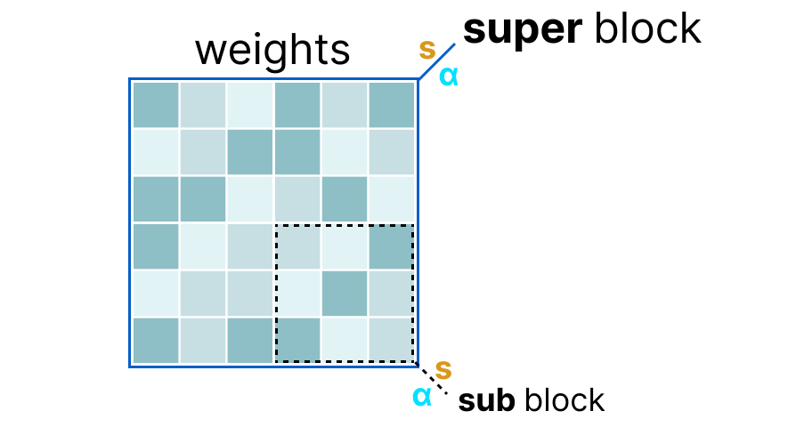
To quantize a given “sub” block, we can use the absmax quantization we used before. Remember that it multiplies a given weight by the scale factor (s):要量化给定的“子”块，我们可以使用之前使用的 absmax 量化。请记住，它将给定的权重乘以比例因子 (s)：

The scale factor is calculated using the information from the “sub” block but is quantized using the information from the “super” block which has its own scale factor:比例因子是使用“子”块的信息计算出来的，但它是使用“超级”块的信息进行量化的，而“超级”块有其自己的比例因子：

This block-wise quantization uses the scale factor (s_super) from the “super” block to quantize the scale factor (s_sub) from the “sub” block.这种块级量化使用来自“超级”块的比例因子 (s_super) 来量化来自“子”块的比例因子 (s_sub)。

The quantization level of each scale factor might differ with the “super” block generally having a higher precision than the scale factor of the “sub” block.每个比例因子的量化级别可能有所不同，“超级”块的精度通常高于“子”块的比例因子。

To illustrate, let’s explore a couple of quantization levels (2-bit, 4-bit, and 6-bit):为了说明这一点，让我们探讨几种量化级别（2 位、4 位和 6 位）：

NOTE: Depending on the quantization type, an additional minimum value (m) is needed to adjust the zero-point. These are quantized the same as the scale factor (s).注意：根据量化类型的不同，可能需要一个额外的最小值 (m) 来调整零点。这些值的量化方式与比例因子 (s) 相同。

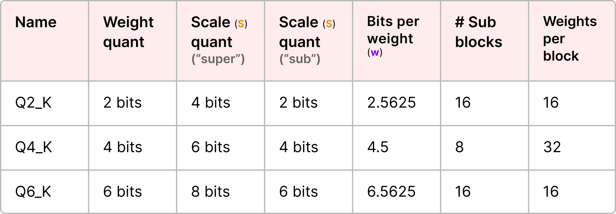
Check out the original pull request for an overview of all quantization levels. Also, see this pull request for more information on quantization using importance matrices.查看原始 pull request 以获取所有量化级别的概述。此外，请参阅此 pull request 以获取有关使用重要性矩阵进行量化的更多信息。

Part 4: Quantization Aware Training

第四部分：量化感知训练 (QAT)

In Part 3, we saw how we could quantize a model after training. A downside to this approach is that this quantization does not consider the actual training process. 在第三部分中，我们了解了如何在训练后量化模型。这种方法的一个缺点是量化过程没有考虑实际的训练过程。

This is where Quantization Aware Training (QAT) comes in. Instead of quantizing a model after it was trained with post-training quantization (PTQ), QAT aims to learn the quantization procedure during training.这就是量化感知训练 (QAT) 的用武之地。QAT 不会在训练后使用训练后量化 (PTQ) 来量化模型，而是旨在在训练期间学习量化过程。

QAT tends to be more accurate than PTQ since the quantization was already considered during training. It works as follows:QAT 往往比 PTQ 更准确，因为量化在训练期间就已经被考虑在内了。其工作原理如下：

During training, so-called “fake” quants are introduced. This is the process of first quantizing the weights to, for example, INT4 and then dequantizing back to FP32:在训练期间，引入了所谓的“伪”量化。这是一个先将权重量化为（例如）INT4，然后再反量化回 FP32 的过程：

This process allows the model to consider the quantization process during training, the calculation of loss, and weight updates.此过程允许模型在训练、损失计算和权重更新期间考虑量化过程。

QAT attempts to explore the loss landscape for “wide” minima to minimize the quantization errors as “narrow” minima tend to result in larger quantization errors.QAT 试图探索损失函数的“宽”极小值区域，以最大限度地减少量化误差，因为“窄”极小值往往会导致更大的量化误差。

For example, imagine if we did not consider quantization during the backward pass. We choose the weight with the smallest loss according to gradient descent. However, that would introduce a larger quantization error if it’s in a “narrow” minima.例如，想象一下如果我们不在反向传播中考虑量化。我们根据梯度下降选择损失最小的权重。然而，如果它处于“窄”极小值中，那将会引入更大的量化误差。

In contrast, if we consider quantization, a different updated weight will be selected in a “wide” minima with a much lower quantization error.相反，如果我们考虑量化，则会在“宽”极小值中选择一个不同的更新权重，其量化误差要小得多。

As such, although PTQ has a lower loss in high precision (e.g., FP32), QAT results in a lower loss in lower precision (e.g., INT4) which is what we aim for.因此，尽管 PTQ 在高精度（如 FP32）下损失更低，但 QAT 在低精度（如 INT4）下能获得更低的损失，这正是我们的目标。

The Era of 1-bit LLMs: BitNet

1 位大语言模型时代：BitNet

Going to 4-bits as we saw before is already quite small but what if we were to reduce it even further?正如我们之前所见，降至 4 位已经很小了，但如果我们进一步减少呢？

This is where BitNet comes in, representing the weights of a model single 1-bit, using either -1 or 1 for a given weight.³ 这就是 BitNet 的用武之地，它将模型的权重表示为 1 位，给定权重仅使用 -1 或 1。

It does so by injecting the quantization process directly into the Transformer architecture.它通过将量化过程直接注入到 Transformer 架构中来实现这一点。

Remember that the Transformer architecture is used as the foundation of most LLMs and is composed of computations that involve linear layers:请记住，Transformer 架构被用作大多数大语言模型的基础，并且由涉及线性层的计算组成：

These linear layers are generally represented with higher precision, like FP16, and are where most of the weights reside.这些线性层通常以高精度（如 FP16）表示，并且是大多数权重所在的地方。

BitNet replaces these linear layers with something they call the BitLlinear:BitNet 用它们称为 BitLinear 的东西替换了这些线性层：

A BitLinear layer works the same as a regular linear layer and calculates the output based on the weights multiplied by the activation. BitLinear 层的工作方式与常规线性层相同，并根据权重乘以激活值来计算输出。

In contrast, a BitLinear layer represents the weights of a model using 1-bit and activations using INT8:相比之下，BitLinear 层使用 1 位表示模型权重，使用 INT8 表示激活值：

A BitLinear layer, like Quantization-Aware Training (QAT) performs a form of “fake” quantization during training to analyze the effect of quantization of the weights and activations:像量化感知训练 (QAT) 一样，BitLinear 层在训练期间执行一种“伪”量化，以分析权重和激活值量化的影响：

NOTE: In the paper they used γ instead of α but since we used a throughout our examples, I’m using that. Also, note that β is not the same as we used in zero-point quantization but the average absolute value.注意：在论文中，他们使用 γ 而不是 α，但由于我们在整个示例中都使用了 α，所以我在这里也使用它。另外，请注意 β 与我们在零点量化中使用的不同，它是绝对值的平均值。

Let’s go through the BitLinear step-by-step.让我们一步步了解 BitLinear。

Weight Quantization

权重量化

While training, the weights are stored in INT8 and then quantized to 1-bit using a basic strategy, called the signum function.在训练期间，权重以 INT8 存储，然后使用一种称为符号函数（signum function）的基本策略量化为 1 位。

In essence, it moves the distribution of weights to be centered around 0 and then assigns everything left to 0 to be -1 and everything to the right to be 1:本质上，它将权重的分布移动到以 0 为中心，然后将所有左侧的值分配为 -1，右侧的值分配为 1：

Additionally, it tracks a value β (average absolute value) that we will use later on for dequantization. 此外，它还会跟踪一个值 β（绝对平均值），我们稍后将在反量化中使用它。

Activation Quantization

激活值量化

To quantize the activations, BitLinear makes use of absmax quantization to convert the activations from FP16 to INT8 as they need to be in higher precision for the matrix multiplication (×). 为了量化激活值，BitLinear 使用 absmax 量化将激活值从 FP16 转换为 INT8，因为它们在矩阵乘法 (×) 中需要更高的精度。

Additionally, it tracks α (highest absolute value) that we will use later on for dequantization.此外，它还会跟踪 α（最高绝对值），我们稍后将在反量化中使用它。

Dequantization

反量化

We tracked α (highest absolute value of activations) and β (average absolute value of weights) as those values will help us dequantize the activations back to FP16.我们跟踪了 α（激活值的最高绝对值）和 β（权重的绝对平均值），因为这些值将帮助我们将激活值反量化回 FP16。

The output activations are rescaled with {α, γ} to dequantize them to the original precision:输出激活值用 {α, γ} 重新缩放，以将其反量化回原始精度：

And that’s it! This procedure is relatively straightforward and allows models to be represented with only two values, either -1 or 1. 就是这样！这个过程相对简单，允许模型仅用两个值（-1 或 1）来表示。

Using this procedure, the authors observed that as the model size grows, the smaller the performance gap between a 1-bit and FP16-trained becomes.使用此过程，作者观察到随着模型规模的增长，1 位训练模型与 FP16 训练模型之间的性能差距会越来越小。

However, this is only for larger models (>30B parameters) and the gab with smaller models is still quite large.然而，这仅适用于大型模型（>30B 参数），小型模型之间的差距仍然相当大。

All Large Language Models are in 1.58 Bits

所有大语言模型都在 1.58 位

BitNet 1.58b was introduced to improve upon the scaling issue previously mentioned.⁴引入 BitNet 1.58b 是为了改进之前提到的缩放问题。

In this new method, every single weight of the model is not just -1 or 1, but can now also take 0 as a value, making it ternary. Interestingly, adding just the 0 greatly improves upon BitNet and allows for much faster computation.在这种新方法中，模型的每一个权重不仅是 -1 或 1，现在还可以取 0 作为值，使其成为三进制。有趣的是，仅仅增加 0 就能极大地改进 BitNet 并实现更快的计算。

The Power of 0

0 的力量

So why is adding 0 such a major improvement?那么为什么增加 0 是一个重大的改进呢？

It has everything to do with matrix multiplication!这与矩阵乘法密切相关！

First, let’s explore how matrix multiplication in general works. When calculating the output, we multiply a weight matrix by an input vector. Below, the first multiplication of the first layer of a weight matrix is visualized:首先，让我们探讨一下矩阵乘法的一般工作原理。在计算输出时，我们将权重矩阵与输入向量相乘。下图直观地展示了权重矩阵第一层的首次乘法运算：

Note that this multiplication involves two actions, multiplying individual weights with the input and then adding them all together.请注意，此乘法过程包含两个动作：将各个权重与输入相乘，然后将它们全部相加。

BitNet 1.58b, in contrast, manages to forego the act of multiplication since ternary weights essentially tell you the following:相比之下，BitNet 1.58b 设法省去了乘法运算，因为三值权重本质上代表了以下含义：

• 1: I want to add this value1：我想加上这个值

• 0: I do not want this value0：我不需要这个值

• -1: I want to subtract this value-1：我想减去这个值

As a result, you only need to perform addition if your weights are quantized to 1.58 bit:因此，如果权重被量化为 1.58 位，你只需要执行加法运算：

Not only can this speed up computation significantly, but it also allows for feature filtering.这不仅能显著加快计算速度，还支持特征过滤。

By setting a given weight to 0 you can now ignore it instead of either adding or subtracting the weights as is the case with 1-bit representations.通过将给定的权重设为 0，你现在可以直接忽略它，而不必像 1 位表示法那样必须执行加法或减法。

Quantization

量化

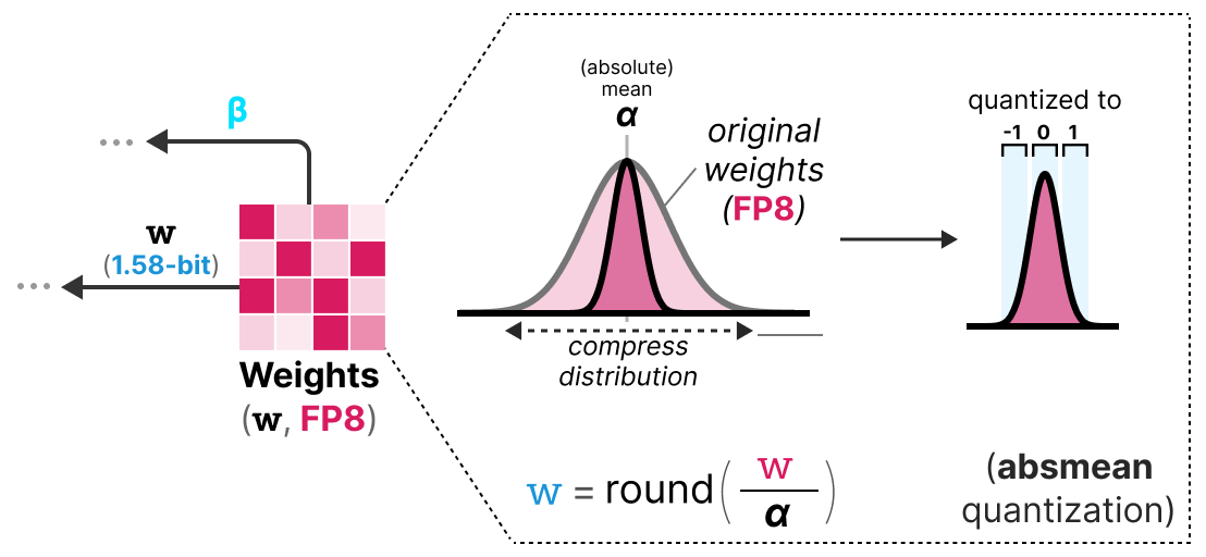
To perform weight quantization BitNet 1.58b uses absmean quantization which is a variation of the absmax quantization that we saw before. 为了执行权重量化，BitNet 1.58b 使用了 absmean 量化，这是我们之前看到的 absmax 量化的一种变体。

It simply compresses the distribution of weights and uses the absolute mean (α) to quantize values. They are then rounded to either -1, 0, or 1:它只是压缩了权重的分布，并使用绝对平均值 (α) 对数值进行量化。然后将它们四舍五入为 -1、0 或 1：

Compared to BitNet the activation quantization is the same except for one thing. Instead of scaling the activations to range [0, 2ᵇ⁻¹], they are now scaled to
[-2ᵇ⁻¹, 2ᵇ⁻¹] instead using absmax quantization.与 BitNet 相比，激活量化的过程几乎相同，只有一点不同。它不再将激活值缩放到 [0, 2ᵇ⁻¹] 范围，而是使用 absmax 量化将其缩放到 [-2ᵇ⁻¹, 2ᵇ⁻¹] 范围。

And that’s it! 1.58-bit quantization required (mostly) two tricks:就是这样！1.58 位量化（主要）利用了两个技巧：

• Adding 0 to create ternary representations [-1, 0, 1]添加 0 以创建三值表示法 [-1, 0, 1]

• absmean quantization for weights用于权重的 absmean 量化

“13B BitNet b1.58 is more efficient, in terms of latency, memory usage, and energy consumption than a 3B FP16 LLM”“在延迟、内存占用和能耗方面，13B BitNet b1.58 比 3B FP16 大语言模型更高效”

As a result, we get lightweight models due to having only 1.58 computationally efficient bits!结果就是，我们得到了轻量级的模型，因为它们只有 1.58 个计算高效的位！

Conclusion

结论

This concludes our journey in quantization! Hopefully, this post gives you a better understanding of the potential of quantization, GPTQ, GGUF, and BitNet. Who knows how small the models will be in the future?!我们的量化之旅到此结束！希望这篇文章能让你更好地理解量化、GPTQ、GGUF 和 BitNet 的潜力。谁知道未来的模型会有多小呢？！

To see more visualizations related to LLMs and to support this newsletter, check out the book I wrote on Large Language Models!

For more information, see the official website. Order the book on Amazon. All code will be uploaded to Github.欲了解更多信息，请查看官方网站。在亚马逊上预订本书。所有代码都将上传到 Github。

Resources

资源

Hopefully, this was an accessible introduction to quantization! If you want to go deeper, I would suggest the following resources:希望这是一篇通俗易懂的量化入门指南！如果你想深入研究，我建议参考以下资源：

• A HuggingFace blog about the LLM.int8() quantization method: you can find the paper here. 一篇关于 LLM.int8() 量化方法的 HuggingFace 博客：你可以在这里找到论文。

• Another great HuggingFace blog about quantization for embeddings.另一篇关于嵌入量化的优秀 HuggingFace 博客。

• A blog about Transformer Math 101, describing the basic math related to computation and memory usage for transformers.一篇关于 Transformer 数学 101 的博客，介绍了与 Transformer 计算和内存使用相关的基础数学知识。

• This and this are two nice resources to calculate the (V)RAM you need for a given model.这个链接和这个链接是计算给定模型所需 (V)RAM 的两个不错资源。

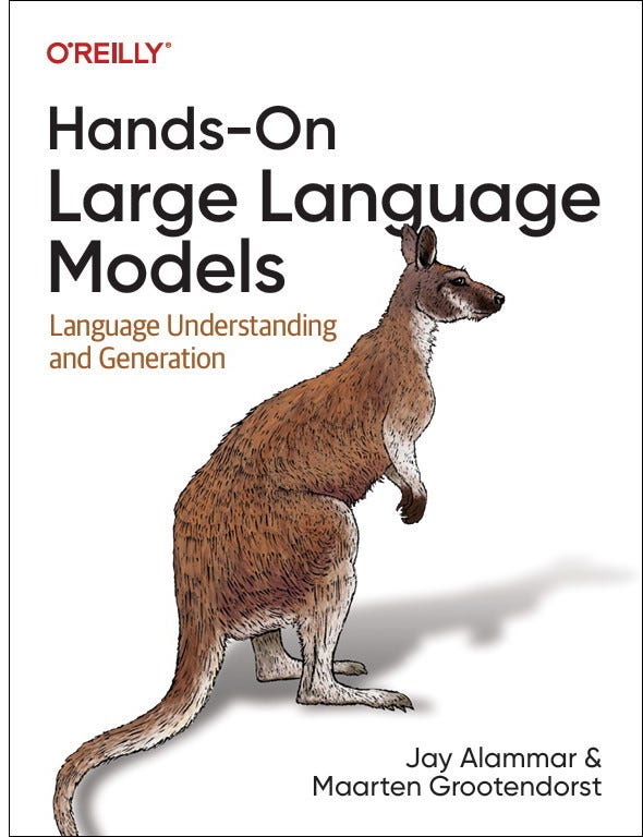
• If you want to know more about QLoRA⁵, a quantization technique for fine-tuning, it is covered extensively in my upcoming book: Hands-On Large Language Models.如果你想了解更多关于 QLoRA5（一种用于微调的量化技术）的信息，我的新书《Hands-On Large Language Models》中有详细介绍。

• A truly amazing YouTube video about GPTQ explained incredibly intuitively. 一个非常棒的 YouTube 视频，以极其直观的方式解释了 GPTQ。

1. Frantar, Elias, et al. "Gptq: Accurate post-training quantization for generative pre-trained transformers." arXiv preprint arXiv:2210.17323 (2022).

2. You can find more about GGUF on their GGML repository here.

3. Wang, Hongyu, et al. "Bitnet: Scaling 1-bit transformers for large language models." arXiv preprint arXiv:2310.11453 (2023).

4. Ma, Shuming, et al. "The era of 1-bit llms: All large language models are in 1.58 bits." arXiv preprint arXiv:2402.17764 (2024).

5. Dettmers, Tim, et al. "Qlora: Efficient finetuning of quantized llms." Advances in Neural Information Processing Systems 36 (2024).