

Generally when performing outlier detection with tabular data, we start by converting the data so that it is either entirely categorical or entirely numeric. There are some exceptions, but for the most part this is necessary: most outlier detection algorithms will assume the data is strictly in one format or the other, and we’ll need to get the data into the format the detector expects. 通常,在使用表格数据进行异常检测时,我们首先会将数据转换为全部分类或全部数值的形式。虽然存在一些例外,但大多数情况下这是必要的:大多数异常检测算法会假设数据严格采用一种格式,我们需要将数据转换为检测器所期望的格式。
If the detector expects categorical data, the numeric features will need to be converted to a categorical format, which generally means binning them. And if the detector expects numeric data, any categorical features need to be numerically encoded. This is the more common scenario (the majority of outlier detection algorithms assume numeric data), and is what we’ll cover in this article. 如果检测器期望分类数据,则需要将数值特征转换为分类格式,通常通过分箱实现。而如果检测器期望数值数据,则需要对分类特征进行数值编码。这是更常见的情况(大多数异常检测算法假设数据为数值型),也是本文将要讨论的内容。
Other articles in the series include: Deep Learning for Outlier Detection on Tabular and Image Data, Distance Metric Learning for Outlier Detection, An Introduction to Using PCA for Outlier Detection, Interpretable Outlier Detection: Frequent Patterns Outlier Factor (FPOF), and Perform Outlier Detection More Effectively Using Subsets of Features. 本系列的其他文章包括:基于深度学习的表格与图像数据异常检测、距离度量学习用于异常检测、使用PCA进行异常检测入门、可解释的异常检测:频繁模式异常因子(FPOF),以及利用特征子集更有效地进行异常检测。
This article also covers some material from the book Outlier Detection in Python.
本文还涵盖了《Python异常检测》一书中的部分内容。
Outlier Detectors异常检测器
Some examples of outlier detection algorithms that assume categorical data include: Frequent Patterns Outlier Factor (FPOF), Association Rules, and Entropy-based methods. Some that work with numeric data include: Isolation Forests, Local Outlier Factor (LOF), kth Nearest Neighbors (kNN), and Elliptic Envelope.一些假设分类数据的异常检测算法示例包括:频繁模式异常因子(FPOF)、关联规则和基于熵的方法。而适用于数值数据的算法包括:孤立森林、局部异常因子(LOF)、k近邻(kNN)和椭圆包络。
If you’re familiar with any outlier detection algorithms, it’s more likely the numeric algorithms, particularly Isolation Forest and LOF; these are probably the most commonly used algorithms. Further, all of the outlier detection algorithms included in scikit-learn and in PYOD (Python Outlier Detection) assume completely numeric data.如果你熟悉任何异常检测算法,更可能是数值型算法,尤其是孤立森林和LOF;它们可能是最常用的算法。此外,scikit-learn和PYOD(Python异常检测库)中包含的所有异常检测算法都假设数据完全是数值型。
At the same time, the great majority of real-world tabular data is actually mixed (containing both numeric and categorical columns), which means, it’s very common when performing outlier detection to need to encode the categorical columns.与此同时,绝大多数现实世界的表格数据实际上是混合型的(同时包含数值和分类列),这意味着在进行异常检测时,通常需要对分类列进行编码。
There is a reason for this: mixed data is more difficult to perform outlier detection on. Working with data of just one type (all categorical or all numeric) does simplify the work of finding the most unusual items in the data.这有其原因:混合数据更难进行异常检测。仅处理单一类型的数据(全部分类或全部数值)确实简化了寻找数据中最异常项的工作。
And, if we work with numeric data, we have the further benefit of being able to view the data geometrically: as points in space. If there are, say, 20 numeric columns in a table, then each row of the data can be viewed as a point in 20-dimensional space. At least, we can conceptually imagine them in 20-d space — the human mind can’t actually picture this. But we can picture 2d and 3d spaces and can extrapolate the general idea: we’re looking for points that are physically very distant from most other points. For example, in 2d, we may have data such as:而且,如果我们处理数值数据,还能进一步以几何方式查看数据:将其视为空间中的点。例如,如果表中有20个数值列,那么每一行数据都可以看作20维空间中的一个点。至少,我们可以在概念上想象它们在20维空间中——人脑实际上无法想象这一点。但我们可以想象二维和三维空间,并推断出一般概念:我们寻找的是那些在物理上远离大多数其他点的点。例如,在二维空间中,我们可能有如下数据:
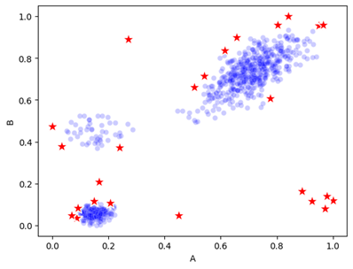
Here, we assume the data has just two features, called A and B, both with numeric values. Each row in the data is drawn either as a blue dot or a red star, with its location based on the values in the A and B columns. The blue dots indicate typical data, and the red stars represent a subset of the points that could be reasonably considered outliers: some points on the fringes of the clusters, and the points outside the clusters (the data has three main clusters, as well as some points outside these).这里,我们假设数据只有两个特征,称为A和B,均为数值。数据中的每一行要么绘制为蓝点,要么绘制为红星,其位置基于A和B列的值。蓝点表示典型数据,红星代表可合理视为异常值的点集:一些位于簇边缘的点,以及簇外的点(数据有三个主要簇,以及一些簇外点)。
This is quite natural in lower dimensions. Things are different in high dimensions, due to what’s called the curse of dimensionality, and we do have to be mindful of that. But, conceptually, the idea of outliers as relatively isolated points in high-dimensional space is fairly straightforward. 这在低维空间中很自然。在高维空间中,由于所谓的“维度灾难”,情况有所不同,我们必须注意这一点。但从概念上讲,将异常值视为高维空间中相对孤立的点这一想法相当直接。
Most numeric outlier detectors work by calculating the distances between each pair of points, and using these distances to identify the points that are most unusual — the points that have few points near them and that are far away from most other points. Though, in practice (for efficiency), the algorithms won’t actually calculate every pairwise distance (some can be skipped where it won’t substantially affect the outlier scores), but in principle, this is what the majority of numeric outlier detectors are doing. 大多数数值异常检测器通过计算每对点之间的距离,并利用这些距离来识别最异常的点——即附近点少且远离大多数其他点的点。尽管在实践中(出于效率考虑),算法不会真正计算每一对距离(某些情况下可以跳过,只要不会显著影响异常分数),但原则上,这是大多数数值异常检测器所做的。
We need, then, ways to convert categorical data to a numeric format that supports this well; that is, that makes it meaningful to calculate distances between rows after encoding the categorical values as numbers.因此,我们需要将分类数据转换为支持这一点的数值格式;也就是说,在将分类值编码为数字后,能够有意义地计算行之间的距离。
Methods to encode categorical data编码分类数据的方法
With prediction problems, the most common encoding methods likely include:在预测问题中,最常见的编码方法可能包括:
- One-hot encoding独热编码
- Ordinal encoding序数编码
- Target encoding目标编码
With outlier detection, the set of options is a bit different, and the strengths and weaknesses of each are also different. Out of the three methods listed here, really only One-hot encoding works well for outlier detection. With outlier detection, the most effective are likely:在异常检测中,可选方法有所不同,每种方法的优缺点也不同。在这三种方法中,实际上只有独热编码适用于异常检测。对于异常检测,最有效的方法可能是:
- One-hot encoding
- Count encoding 计数编码
I’ll describe how each works, and why some work better than others for outlier detection. And I’ll explain why Count encoding (which is rarely used with prediction problems) can be quite useful with outlier detection.我将描述每种方法的工作原理,以及为什么有些方法在异常检测中效果更好。并解释为什么计数编码(在预测问题中很少使用)在异常检测中非常有用。
I should also say, besides these encoding methods, there are several others that can be useful for prediction. An excellent library for encoding methods is Category Encoders. This will likely cover any of the methods you will need. Many of the methods provided, though, such as Target encoding and CatBoost encoding, require a target column, which is normally not available with outlier detection. 我还应该提到,除了这些编码方法,还有其他几种方法可用于预测。一个优秀的编码方法库是Category Encoders。它很可能涵盖你需要的所有方法。不过,其中许多方法,如目标编码和CatBoost编码,需要一个目标列,这在异常检测中通常不可用。
For example, if we had a table representing historical information about customers of a business, there may be a categorical column for “Last Product Purchased” and a target column called “Will Churn in next 6 Months”. The “Last Product Purchased” column may have the distinct values: “Product A”, “Product B”, and “Product C”. To encode these, we can calculate how often the target column has value True for each value (in the training data), possibly encoding these as 0.12, 0.43, 0.02 (meaning, when the ‘Last Product Purchased’ is Product A, 12% of the time the Target column is True, and the client churns in the next 6 months; similarly for Product B (43%) and Product C (2%)). 例如,如果我们有一个代表客户历史信息的表格,可能有一个分类列“最后购买的产品”和一个目标列“未来6个月内是否会流失”。“最后购买的产品”列可能有不同的值:“产品A”、“产品B”和“产品C”。为了编码这些值,我们可以计算每个值(在训练数据中)目标列为真的频率,可能编码为0.12、0.43、0.02(这意味着,当“最后购买的产品”为产品A时,目标列为真的概率为12%,客户在未来6个月内流失;产品B为43%,产品C为2%)。
But with outlier detection, we’re working in a strictly unsupervised environment: there is no ground truth value for how outlierish each row is, and so no way to set a Target column. We can use only unsupervised encoding methods, including One-hot and Count encoding. 但在异常检测中,我们是在完全无监督的环境下工作:没有每行异常程度的真实值,因此无法设置目标列。我们只能使用无监督编码方法,包括独热编码和计数编码。
One-hot encoding
To look at One-hot encoding, I’ll start by describing how it is done, and then will look at how it works with distance calculations. Let’s assume we start with a table such as the following:为了了解独热编码,我将首先描述其实现方式,然后探讨它如何与距离计算配合。假设我们从如下表格开始:
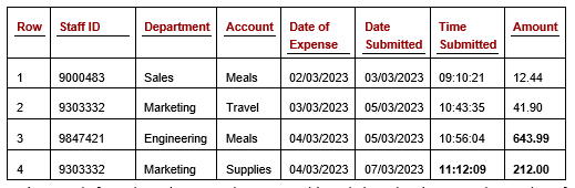 Table 1: Staff Expenses table表1:员工费用表
This table describes staff expenses, with one row per expense claim. Assuming we plan to use one or more numeric outlier detectors, we’ll need to convert the categorical columns (Staff ID, Department, and Account) to numbers. 该表描述了员工费用,每行代表一笔费用报销。假设我们计划使用一个或多个数值异常检测器,我们需要将分类列(员工ID、部门和账户)转换为数字。
The Date and Time columns will also need to be converted to numeric values. Outlier Detection in Python covers working with date and time data. I don’t have space in this article, but will say quickly that they can be converted in a number of ways. One simple method is by calculating the time since some starting point (referred to as the epoch). The minimum date or time in the column may be used, or some other date that represents a logical starting point. 日期和时间列也需要转换为数值。《Python异常检测》涵盖了日期和时间数据的处理。本文篇幅有限,但简要说明一下:它们可以通过多种方式转换。一种简单的方法是计算自某个起始点(称为纪元)以来的时间。可以使用列中的最小日期或时间,或其他代表逻辑起点的日期。
Let’s say we use January 1, 1990. All dates can then be represented as the number of days since that point. We do, though, also wish to capture more information about the dates, such as the day of the week (this may be relevant, for example, if staff expenses for weekends are unusual), if they fall on a holiday, and so on, so we may wish to look at other encoding methods as well. For this article, though, we’ll focus just on categorical columns. 假设我们使用1990年1月1日。所有日期都可以表示为自该点以来的天数。不过,我们还需要捕获关于日期的更多信息,例如星期几(如果周末的员工费用异常,这可能相关)、是否在节假日等,因此我们可能还需要考虑其他编码方法。但本文中,我们只关注分类列。
If we consider, for the moment, just the Department column, by One-hot encoding this column, we replace the column with a series of new columns, one for each unique value in the column. Let’s assume the column had five distinct values: Sales, Marketing, Engineering, HR, and Communications. We would then have five new columns representing these values, such as in the following table (Table 2). This shows just the Staff ID column, and the new columns related to Department. (The other columns would be present as well, but are skipped here for simplicity. A similar set of columns would be created, for example, for the Account column).如果我们暂时只考虑部门列,通过独热编码该列,我们将该列替换为一系列新列,每列对应列中的一个唯一值。假设该列有五个不同的值:销售、市场、工程、人力资源和通信。那么我们将有五个新列代表这些值,如下表(表2)所示。这里只显示了员工ID列和与部门相关的新列。(其他列也会存在,但为简单起见此处省略。例如,账户列也会创建类似的一组列)。
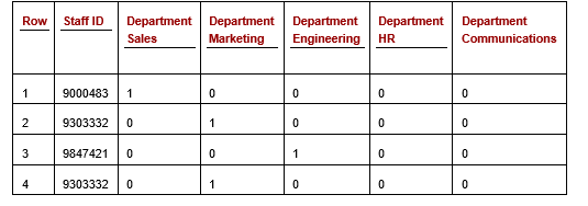 Table 2: Staff Expenses table with the Department column one-hot encoded (some columns not shown)表2:部门列经过独热编码的员工费用表(部分列未显示)
Each of the cells in the one-hot Department columns will have a value of either 0 or 1, indicating if that is the correct value for this row. We see here in the first row, an expense claim for Staff 9000483, who is in Sales. Given that, the column for ‘Department Sales’ has a 1 and the other columns related to the Department have a 0. Similarly, for each other row: exactly one of the Department columns will have a 1, and all others a 0.独热编码部门列中的每个单元格的值将为0或1,表示该行是否属于该值。我们看到第一行,员工9000483的费用报销,该员工属于销售部门。因此,“部门_销售”列为1,其他与部门相关的列为0。类似地,对于其他每一行:恰好有一个部门列为1,其余为0。
One-hot encoding is very commonly used for outlier detection and can be a good choice when a feature has low cardinality. It can, though, break down somewhat where the column has very high cardinality. For example, if the Department column in the original staff expenses table had 100 distinct values, it would result in 100 new columns being created, which can create a table that’s difficult to work with. I’ll show below, though, that it’s actually no worse for distance calculations than with low-cardinality situations, and so may still be workable. 独热编码在异常检测中非常常用,当特征基数较低时是一个不错的选择。然而,当列基数非常高时,它可能会出现问题。例如,如果原始员工费用表中的部门列有100个不同的值,则会创建100个新列,这可能导致表格难以处理。不过,我将在下面展示,对于距离计算而言,它实际上并不比低基数情况更差,因此可能仍然可行。
At the same time, high-cardinality columns are not generally as useful for outlier detection as low-cardinality columns. For this reason, we may not want to include the Staff Id column in the our outlier detection process. Though we also may: it may still be informative and useful to include — for example, if we wish to find expenses that are large for that staff, staff that have unusual numbers of expenses, staff that have many similar expenses close in time and so on. 同时,高基数列通常不如低基数列对异常检测有用。因此,我们可能不希望将员工ID列包含在异常检测过程中。不过,我们也可以包含它——它可能仍然具有信息量且有用——例如,如果我们希望找出该员工的大额费用、异常数量的费用、时间上接近的相似费用等。
One-hot encoding with Isolation Forest使用孤立森林的独热编码
How much of a problem generating many additional columns depends on the outlier detection algorithm. One of the most well-used outlier detection algorithms is Isolation Forest, which does not use distance calculations. Instead, it identifies low-density subspaces in the feature space and flags the rows that appear in these. Which means, it’s still looking for points that are far from other points, but does so without calculating the distances between points. 生成许多额外列的问题程度取决于异常检测算法。最常用的异常检测算法之一是孤立森林,它不使用距离计算。相反,它识别特征空间中的低密度子空间,并标记出现在这些子空间中的行。这意味着,它仍然在寻找远离其他点的点,但无需计算点之间的距离。
I can’t get into the details of Isolation Forest here (hopefully a future article, though), but will say quickly that if a single column is expanded into many columns after encoding (as with One-hot encoding and some other encoding schemes), those columns will be overrepresented in the analysis of the Isolation Forest algorithm, which we probably don’t want.我无法在此深入探讨孤立森林的细节(希望未来有文章介绍),但简要说明:如果单个列在编码后扩展为多个列(如独热编码和其他一些编码方案),这些列将在孤立森林算法的分析中被过度代表,这可能是我们不希望的。
Due to some interesting details of how the Isolation Forest algorithm works internally, it’s actually usually most effective with Isolation Forests to use Ordinal encoding. Having said that, Isolation Forest is one of the very few outlier detection algorithms where this is true — with most other detectors Ordinal encoding works quite poorly. I’ll describe it below and explain why that’s the case. 由于孤立森林算法内部工作的一些有趣细节,实际上,对于孤立森林,使用序数编码通常最有效。话虽如此,孤立森林是极少数适用此规则的异常检测算法之一——对于大多数其他检测器,序数编码效果很差。我将在下面描述并解释原因。
Distance calculations with One-hot encoding使用独热编码的距离计算
Most numeric outlier detectors, however, are based on calculating and assessing the distances between points (or between each point and the data center, or cluster centers). This includes: Local Outlier Factor, k-Nearest Neighbors, Radius, Gaussian Mixture Models, KDE (Kernel Density Estimation), Elliptic Envelope, One-Class Support Vector (OCSVM), and numerous others.然而,大多数数值异常检测器基于计算和评估点之间的距离(或每个点到数据中心或簇中心的距离)。这包括:局部异常因子、k近邻、半径、高斯混合模型、KDE(核密度估计)、椭圆包络、一类支持向量机(OCSVM)等。
The encoding method will affect the distances calculated, and consequently, the outlier scores given to each row. One-hot encoding does usually work relatively well with outlier detection for most numeric detectors (including those based on distance calculations), but it does have one negative: as with Isolation Forests, One-hot encoding results in categorical features being overrepresented in distance calculations, though the effect is less severe than with Isolation Forests.编码方法会影响计算的距离,从而影响每行的异常分数。独热编码通常对大多数数值检测器(包括基于距离的检测器)的异常检测效果相对较好,但它有一个缺点:与孤立森林类似,独热编码会导致分类特征在距离计算中被过度代表,尽管影响不如孤立森林严重。
As an example, consider the following table (Table 3), which shows a dataset with four rows and two features. The Colour column has five values (with two present in the current data) — red, blue, green, white, and yellow. The size column has two values: big and small.例如,考虑下表(表3),该表显示了一个包含四行和两个特征的数据集。颜色列有五个值(当前数据中出现两个)——红色、蓝色、绿色、白色和黄色。大小列有两个值:大和小。
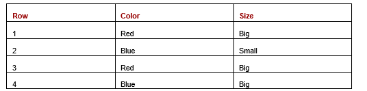 Table 3: Dataset with Colour and Size features表3:包含颜色和大小特征的数据集
The pair-wise distances between the four rows are shown in the next table (Table 4). There are many distance calculations we could use; this method leaves the data as categorical (we don’t do any numeric encoding yet) and measures the distance between two rows as the number of values that are different.四行之间的成对距离如下表(表4)所示。我们可以使用多种距离计算方法;此方法将数据保留为分类形式(尚未进行数值编码),并测量两行之间不同值的数量。
As there are two features, a pair of rows can have a distance of zero, one, or two (they can have zero, one, or both features different). The table shows only the distances between each unique pair of rows and shows each distance only once (e.g. between Row 1 and Row 2, but between Row 2 and Row 1, which would be the same; and not between Row 1 and itself), so shows values only above the main diagonal.由于有两个特征,一对行的距离可以是0、1或2(它们可以有0、1或两个特征不同)。该表仅显示每对唯一行之间的距离,并且每个距离只显示一次(例如,行1和行2之间,但行2和行1相同;不包括行1自身),因此仅显示主对角线以上的值。
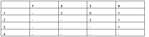 Table 4: Distances between each pair of rows using a distance metric that considers if features have the same value or not.表4:使用考虑特征值是否相同的距离度量计算的行对距离。
If we One-hot encode the original data (from Table 3), we get:如果我们对原始数据(来自表3)进行独热编码,得到:
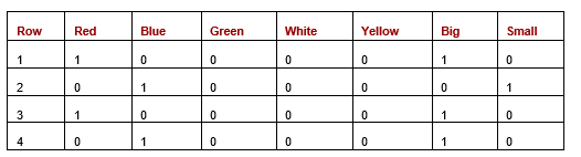 Table 5: Dataset after one-hot encoding表5:独热编码后的数据集
If we calculate the pair-wise distances between the rows using one-hot encoding and either Manhattan or Euclidean distances, we have the distances shown in the next table. In this case, as all values are 0 or 1, the Manhattan and Euclidean distances are actually the same.如果我们使用独热编码并计算曼哈顿距离或欧氏距离,得到下表中的距离。在这种情况下,由于所有值都是0或1,曼哈顿距离和欧氏距离实际上相同。
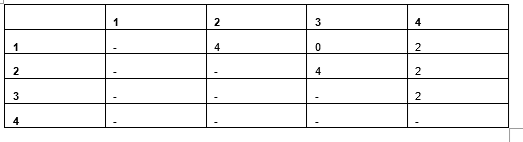 Table 6: Pairwise Manhattan/Euclidean distances表6:成对曼哈顿/欧氏距离
Using Manhattan (or Euclidean) distance measures, the distances are proportional to when using a count of the number of values matching (as we did for Table 4), but the values are double: when two values in the original data mismatch, there will be two cells in the one-hot encoding mismatched. This is not usually a problem when working with purely categorical data, but it does create an undesirable situation where we have mixed data.使用曼哈顿(或欧氏)距离度量时,距离与使用匹配值计数(如表4所示)成比例,但数值加倍:当原始数据中的两个值不匹配时,独热编码中会有两个单元格不匹配。这在处理纯分类数据时通常不是问题,但在处理混合数据时会产生不理想的情况。
Consider Table 7 with two features: Color and Weight, where Weight is numeric.考虑表7,其中有两个特征:颜色和重量,重量为数值。
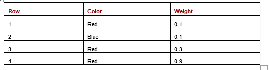 Table 7: Dataset with one categorical and one numeric feature
Once one-hot encoded, we have Table 8:表7:包含一个分类特征和一个数值特征的数据集。经过独热编码后,得到表8:
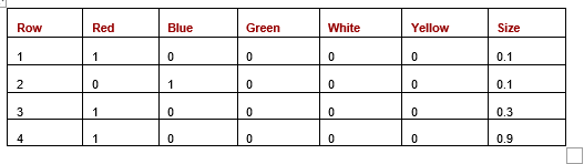 Table 8: One-hot encoding with one categorical and one numeric feature表8:包含一个分类特征和一个数值特征的独热编码
Here, when we calculate Euclidean distances between the rows. (We can also use Manhattan, Canberra, or any other distance metric, but for this example, use Euclidean). We show the Euclidean distances in the following table (Table 9):这里,我们计算行之间的欧氏距离。(我们也可以使用曼哈顿、堪培拉或其他距离度量,但本例使用欧氏距离)。欧氏距离如下表(表9)所示:
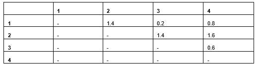 Table 9: Distances based on Euclidean distances表9:基于欧氏距离的距离
Rows 1 and 2 differ in the Colour (having the same weight) and have a Euclidean distance of 1.4. Rows 3 and 4 are different in weight (having the same color) and have a Euclidean distance of just 0.6. We can see the difference in Colour is more significant than Weight in determining the distance, though likely it should not be.行1和行2在颜色上不同(重量相同),欧氏距离为1.4。行3和行4在重量上不同(颜色相同),欧氏距离仅为0.6。我们可以看到,颜色差异在决定距离时比重量更重要,尽管可能不应该如此。
There are two factors that give categorical features more importance here than numeric. The first is that matches versus non-matches affect two one-hot columns, while the differences in numeric values affect only a single column. The second is that distances in binary columns are larger than in numeric features. Here, Row 1 and Row 4 have Weight values of 0.1 and 0.9, which have a significant difference of 0.8 — but this is less than the difference in two mismatching categorical values, which will be 2.0 (given that two binary columns will mismatch).有两个因素使分类特征在此比数值特征更重要。首先,匹配与不匹配影响两个独热列,而数值差异仅影响一个列。其次,二元列中的距离大于数值特征中的距离。这里,行1和行4的重量值分别为0.1和0.9,差异显著为0.8——但这小于两个不匹配分类值的差异,后者将为2.0(因为两个二元列不匹配)。
An example working with Manhattan and Euclidean distances is shown in the following listing. In the first case, we create a pair of vectors representing the first two rows from the previous data, with five one-hot columns for Colour and one column for Weight. We then create another pair of vectors to simulate what it would look like if the cardinality of Color were instead 2, using only two binary columns.以下列表展示了使用曼哈顿和欧氏距离的示例。在第一种情况下,我们创建一对向量,代表前两行数据,包含五个颜色独热列和一个重量列。然后,我们创建另一对向量,模拟颜色基数仅为2的情况,仅使用两个二元列。
Here we show some code testing the Manhattan and Euclidean distances:这里我们展示了一些测试曼哈顿和欧氏距离的代码:
from sklearn.metrics.pairwise import euclidean_distances, \
manhattan_distances

# Creates data simulating two rows where five binary columns are
# used for one categorical
row_1 = [1, 0, 0, 0, 0, 0.1]
row_2 = [0, 1, 0, 0, 0, 0.1]
print(manhattan_distances([row_1], [row_2]))
print(euclidean_distances([row_1], [row_2]))

# Creates similar data but with two binary columns for one
# categorical column
row_1 = [1, 0, 0.1]
row_2 = [0, 1, 0.2]
print(manhattan_distances([row_1], [row_2]))
print(euclidean_distances([row_1], [row_2]))
Interestingly, in both cases, the two rows have a Manhattan distance of 2.1 and Euclidean of 1.4: where we test using only two binary features for Colour instead of five, the distances are the same. Similarly, increasing the cardinality (using more than five binary columns to represent color) does not affect the distance measures. Regardless of how many one-hot columns there are related to Colour, if two rows have the same colour, there will be 0 differences; and if they have different colours, there will be 2 differences (all other columns will be zero, and therefore matching). 有趣的是,在两种情况下,两行的曼哈顿距离均为2.1,欧氏距离均为1.4:当我们仅使用两个二元特征表示颜色而不是五个时,距离相同。类似地,增加基数(使用超过五个二元列表示颜色)不会影响距离度量。无论有多少个与颜色相关的独热列,如果两行颜色相同,则差异为0;如果颜色不同,则差异为2(所有其他列均为0,因此匹配)。
So, there is, as noted, an imbalance between categorical and numeric features, but it is not made worse by the cardinality of the categorical features.因此,如前所述,分类特征和数值特征之间存在不平衡,但不会因分类特征的基数而恶化。
My suggestion, to reduce the over-emphasis in distance calculations, is to replace the 1.0 values in the one-hot columns with 0.25. This will result in rows with different values having a total difference (with respect to that original column) of 0.5 instead of 2.0, putting it more in the same scale as the numeric features.我的建议是,为了减少距离计算中的过度强调,将独热列中的1.0值替换为0.25。这将使具有不同值的行相对于原始列的总差异从2.0降至0.5,使其更接近数值特征的尺度。
Ordinal encoding
Ordinal encoding works by simply giving each unique value in a categorical column a unique number. In the example above, we may give the values in the Colour column values such as:序数编码通过为分类列中的每个唯一值赋予一个唯一数字来工作。在上面的例子中,我们可以为颜色列中的值赋予如下值:
red: 1
blue: 2
green: 3
white: 4
yellow: 5红色:1 蓝色:2 绿色:3 白色:4 黄色:5
So all values of “red” would be replaced by 1, and so on. Similarly for the Size column: we can replace ‘small” with, say, 1 and “big” with 2, or with any other numeric values. 因此,所有“红色”值将被替换为1,依此类推。对于大小列,我们可以将“小”替换为1,“大”替换为2,或任何其他数值。
As indicated, this does actually work well for Isolation Forest. But it doesn’t tend to work well for most other numeric outlier detectors, including those based on distances. Ordinal encoding does avoid creating additional columns: each categorical column is translated into a single numeric column. But, the distance calculations will become meaningless. 如前所述,这实际上对孤立森林效果很好。但对于大多数其他数值异常检测器,包括基于距离的检测器,效果通常不佳。序数编码确实避免了创建额外列:每个分类列被转换为单个数值列。但是,距离计算将变得毫无意义。
Using the values above, rows with value yellow would be considered 4.0 away from those with value red, while those with value white would only be 1.0 away from rows with yellow, which make little sense. The distances end up completely arbitrary. 使用上述值,值为黄色的行与值为红色的行之间的距离将被视为4.0,而值为白色的行与黄色的行之间的距离仅为1.0,这几乎没有意义。距离最终变得完全任意。
Count encoding
Count encoding is actually much more important as an encoding technique with outlier detection than with prediction. As with Ordinal encoding, it coverts each categorical column to a single numeric column, but with Count encoding, does so in a way that the numeric values aren’t random; they have meaning, and meaning that’s relevant to outlier detection. 计数编码实际上在异常检测中比在预测中更为重要。与序数编码一样,它将每个分类列转换为单个数值列,但计数编码以非随机的方式赋予数值,这些数值具有意义,并且与异常检测相关。
Count encoding also produces numeric values that are straightforward for distance calculations.计数编码还产生易于进行距离计算的数值。
With Count encoding, the numeric values generated represent the frequency of the value (rare values will be given small values and common values large values), which has some real information value when working with outlier detection.使用计数编码时,生成的数值代表该值的频率(稀有值将被赋予小值,常见值被赋予大值),这在异常检测中具有实际信息价值。
Taking a look at the Staff Expenses table, if we have a distribution of Department values such as:查看员工费用表,如果我们有部门值的分布如下:
Sales: 1,000
Marketing: 500
Engineering: 100
HR: 10
Communications: 3销售:1,000 市场:500 工程:100 人力资源:10 通信:3
Then, these counts will be the encodings. That is, 1,000 records (those for Sales) will be given value 1,000; 500 will have value 500; and so on. This has the advantage that it can encode values such that rare values tend to be far from other values. In this case, the values 10 and 3 are close to each other, which means these 13 records will be close to each other, but there are still only 13 of them, and they will be far from the other 1,600 records. The value 1,000 is distant from the other values, but there are 1,000 records with this encoding, and so these 1000 records are each close to 999 others, and would then not be flagged as outliers.那么,这些计数就是编码。也就是说,1,000条记录(销售部门)将被赋予值1,000;500条记录将被赋予值500;依此类推。这具有优势,可以编码值,使稀有值往往远离其他值。在这种情况下,值10和3彼此接近,这意味着这13条记录彼此接近,但它们仍然只有13条,并且远离其他1,600条记录。值1,000远离其他值,但有1,000条记录具有此编码,因此这1,000条记录各自接近其他999条记录,因此不会被标记为异常值。
In the following code, using these values, we generate a simple, single-feature dataset representing the department and create a Local Outlier Factor (LOF) detector to assess this. When working with multiple columns, it is necessary to scale any Count-encoded features to ensure all features are on the same scale, but as this example contains only a single feature, this step may be skipped. The LOF is able to correctly identify the rare values as outliers: the 13 rare values are given prediction –1 (indicating outliers in the scikit-learn implementation), while all others are predicted as 1 (indicating inliers).在以下代码中,使用这些值,我们生成一个简单的单特征数据集,代表部门,并创建一个局部异常因子(LOF)检测器进行评估。当处理多个列时,需要对任何计数编码的特征进行缩放,以确保所有特征在同一尺度上,但此示例仅包含一个特征,因此可以跳过此步骤。LOF能够正确识别稀有值为异常值:13个稀有值被预测为–1(在scikit-learn实现中表示异常值),而所有其他值被预测为1(表示正常值)。
import numpy as np
import pandas as pd
from sklearn.neighbors import LocalOutlierFactor

# Creates a dataset with a single categorical column
vals = np.array(['Sales']*1000 + ['Marketing']*500 + ['Engineering']*100 +
['HR']*10 + ['Communications']*3)

# Count-encode the column
df = pd.DataFrame({"C1": vals})
vc = df['C1'].value_counts()
map = {x:y for x,y in zip(vc.index, vc.values)}
df['Ordinal C1'] = df['C1'].map(map)

# Uses LOF to determine the outliers in the column
clf = LocalOutlierFactor(contamination=0.01)
df['LOF Score'] = clf.fit_predict(df[['Ordinal C1']])
One thing to note about Count encoding is that it can give multiple original values the same numeric code if they happen to have the same count. For example, if Sales and Marketing both had 1000 rows, they would both be given an encoding of 1000. Or if Sales had 1000 and Marketing had 1001, they would be given nearly the same encoding. For most detectors, this is not an issue, but again, Isolation Forest is a bit different and it’s better to be able to distinguish values that actually are distinct, which is possible with Ordinal encoding. 关于计数编码需要注意的一点是,如果多个原始值恰好具有相同的计数,则它们可能获得相同的数值代码。例如,如果销售和市场都有1000行,则它们都将被编码为1000。或者,如果销售有1000行,市场有1001行,则它们将被赋予几乎相同的编码。对于大多数检测器,这不是问题,但孤立森林又有所不同,最好能够区分实际不同的值,而序数编码可以实现这一点。
Determining the best encoding method确定最佳编码方法
Which encoding method works best will vary based on the dataset, the outlier detection algorithm, and the types of outliers you wish to find. Unfortunately, like many things in data science, there is no definitive answer as to what’s best; each method can be preferred at times. And, in some cases, it may actually work best to use different encodings for different features.哪种编码方法效果最好,将因数据集、异常检测算法以及您希望发现的异常类型而异。不幸的是,与数据科学中的许多事情一样,没有明确的答案;每种方法有时都可能更优。并且,在某些情况下,对不同特征使用不同的编码方法可能效果最好。
As is a common theme with outlier detection, it can be useful to take an ensemble approach, where rows are encoded in multiple ways. The truly anomalous rows will stand out as outliers using each encoding method, while the more mildly anomalous will possibly stand out just using one or another encoding method. 正如异常检测中常见的主题,采用集成方法可能很有用,即对行进行多种方式的编码。真正异常的行将在每种编码方法下都突出显示为异常值,而较轻微异常的行可能仅通过一种或另一种编码方法突出显示。
Choosing an encoding method can be easier with prediction problems. With prediction problems, we usually have a validation set and can simply try different encoding methods and determine experimentally which works best. With outlier detection, though, the problems are usually completely unsupervised (again, there is no target column as there is no ground truth as to how outlierish each row is). Which means it’s more difficult to evaluate the encoding methods used. We can, though, use a technique for evaluating outlier detection systems known as Doping.对于预测问题,选择编码方法更容易。对于预测问题,我们通常有一个验证集,可以简单地尝试不同的编码方法,并通过实验确定哪种效果最好。然而,对于异常检测,问题通常完全是无监督的(再次强调,没有目标列,因为没有每行异常程度的真实值)。这意味着评估所使用的编码方法更加困难。不过,我们可以使用一种称为“掺杂”的技术来评估异常检测系统。
As well, where the outlier detection system runs over time, it may be possible to collect labeled data and use this to evaluate different preprocessing methods including the encoding of the categorical columns. 此外,如果异常检测系统随时间运行,可能可以收集标记数据,并用其评估不同的预处理方法,包括分类列的编码。
Scaling缩放
If we were working with data that was completely numeric to start with, we wouldn’t need to encode any categorical columns, but we would still need to scale the data, at least with most numeric outlier detectors. Again, Isolation Forest is one of the exceptions, but any based on distance calculations do require that each dimension (each feature) is on the same scale. Otherwise the distances between points (or between the points and cluster centers, etc.) will be dominated by features that happen to be on larger scales.如果我们处理的数据最初完全是数值型,则无需对任何分类列进行编码,但我们仍然需要缩放数据,至少对于大多数数值异常检测器是如此。再次强调,孤立森林是例外之一,但任何基于距离计算的检测器都要求每个维度(每个特征)处于同一尺度。否则,点之间的距离(或点到簇中心的距离等)将由恰好处于较大尺度的特征主导。
The same is true for any categorical columns after encoding. Regardless of the encoding method used, the new numeric features may now be on different scales than the features that were already numeric (and the converted date or time features). And, if different encoding methods are used for different categorical columns, then even these columns may be on different scales as each other.对于编码后的任何分类列也是如此。无论使用何种编码方法,新的数值特征现在可能与原本就是数值的特征(以及转换后的日期或时间特征)处于不同尺度。并且,如果对不同分类列使用了不同的编码方法,那么这些列之间也可能处于不同尺度。
Scaling these columns uses the same methods as numeric columns — we just have to ensure we include these new columns. The specifics of doing this will hopefully be covered in a future article, but quickly: we usually use either a min-max, robust z-scaling, or spline scaling for this. 对这些列进行缩放使用与数值列相同的方法——我们只需确保包含这些新列。具体细节希望在未来文章中介绍,但简要说明:我们通常使用最小-最大缩放、稳健z分数缩放或样条缩放。
All images were by the author所有图片均由作者提供


